may not bother. The average number of calls received in a day is 70.

You are asked to help to put the manager's mind at rest by developing a model to simulate the telephone calls. Use your model to estimate the following.

1.The percentage of time for which zero, one, two and three lines are engaged.

2.The percentage of customers who are put off.

How would you adapt the model if the office had an extra line installed? What extra information would you need to improve the model?

7.6 Packages and simulation languages

As you will have gathered from the previous sections, simulation is essentially an experimental technique in that models are set up and ‘run’ to see what happens. It makes things much easier if the ‘running’ happens inside a computer and it is not surprising that there is a lot of computer software available for constructing and running stochastic simulation models.

The software can be divided into simulation packages and simulation languages. The distinction is that a package will have some form of user interface which will allow you to define your model either by giving responses to questions asked in ordinary English or by making selections from prepared menus. A simulation language, on the other hand, is a specially written high-level language in which you will write your model as a sequence of statements.

Both types of software offer the facilities normally required in discrete simulation such as the generation of pseudo-random numbers for any desired statistical distribution, the collection and summary of data from runs and the statistical analysis and presentation of results. The disadvantage of a simulation language is that you have a new language to learn, which takes up some time. The disadvantage of a simulation package is that it tends to be very convenient for simulating a particular class of problem (for which it has been designed) but very difficult to use on a problem of a completely different kind.

A wide variety of packages and simulation languages are available, differing in their power, flexibility and ease of use. At present the most widely used are WITNESS and SIMULA. You can of course write your own simulation programs in whatever language you choose but the fact that all stochastic simulations involve common elements such as generating random numbers,

finding the next event and updating queues means that you will, to some extent, be constantly ‘reinventing the wheel’.

It is quite adequate to run simple simulation problems using a spreadsheet package (such as EXCEL) as indicated in chapter 2, Example 2.9.

Summary

In this chapter, we have taken a superficial look at a very important type of modelling, namely modelling involving random numbers. This is a very large area and what we have described is merely a brief introduction. There are two different approaches which can be taken in modelling of this type.

1. The analytic approach is to use the theory and functions of mathematical statistics.

2.The simulation approach is to create a model having the required structure and then to use a random-number generator to activate the model. This is often referred to as ‘discrete event simulation’ or ‘stochastic simulation’ and is commonly ‘event-driven’ rather than ‘time-driven’.

The type 1 approach becomes very difficult, once a model acquires a reasonable amount of complexity. The type 2 approach has the disadvantage that several runs are necessary and the results obtained are statistical in nature.

Event-driven simulations can be done by hand but become rather tedious and it is usual to turn to computer software for help. Many specially designed software packages are available for carrying out discrete event simulations. The common uses of simulation models are to investigate the efficiency of proposed new systems or alterations to existing systems. A careful study of the results obtained is necessary and, used sensibly, simulation models can save a great deal of expense since experiments are far cheaper to carry out on models than in the real world.

CHAPTER 8

Using Data

Aims and objectives

In this chapter we discuss how empirical models can be developed from data and also how theoretical models can be fitted to data by choosing appropriate values of parameters.

8.1 Introduction

It is possible to build our mathematical models out of the abstract concepts of mathematics using simply pen and paper or blackboard and chalk. During the model-building activity, we are in a dream world of idealisations and imagination but the real world is still somewhere in the background. If our models are to be more than just curiosities of interest only to mathematicians, they must be made to confront reality and it is through data or conclusions made from data that this confrontation occurs.

By data we mean any facts, measurements or observations which have been collected in the real world. They may well be inaccurate and imperfect but, as far as we can tell, they represent the truth with which our models have to be compared. Interaction between models and data occurs in a number of ways, amongst which are the following.

1.Data can be useful in suggesting models or parts of models during the development stage when we are trying to form our ideas. Some models (referred to as ‘empirical’) can even be based entirely on data. Examples of simple empirical models are given in section 8.3.

2.Data are needed to estimate the values of parameters appearing in a model. This process of estimating particular parameter values for a particular application is sometimes called ‘calibrating’ a model. In section 8.4, we look at some of the methods that can be used and some of the problems involved.

3.Data are needed to test a model, i.e. to check whether our model's predictions correspond reasonably well to what is observed in the real world. We may also wish to choose the best out of a number of alternative models.

8.2Data collection

When you are given a modelling problem, there may be some data that go with it and in some cases you may have to use what you are given and no more. Very often, however, there is the possibility or the need to obtain more data. The task of collecting such data almost invariably turns out to be harder than you think. The questions that you have to try and answer are as follows.

1.Exactly what data are needed? You will probably have to proceed well into the modelling process before you are able to decide what are the relevant data for your particular problem. It is quite possible that you already have more data than you need and you will have to exercise your judgement in throwing away irrelevant or redundant information.

2.How can the relevant data be obtained? You may have to go back to the person or persons who gave you the problem and ask for the data that you need. The data may already be available or it may be necessary to do further experiments. Another common possibility is that your local or college library will be able to guide you to published sources containing the data that you need. In some cases, you may have to collect the data yourself and, depending on the type of model,

this may involve you in activities such as designing questionnaires for statistical surveys or making scientific measurements.

3.In what form do you need the data? If there is a large volume of data, you may want to reduce it by carrying out a statistical summary involving, for example, calculations of means, standard deviations, percentages and histograms. Do not forget to make a note of your sources of data, including dates. These will be needed when you come to write up your report (see chapter 10).

Exercises

For the following exercises, you will need to decide

1.exactly what data are needed (the problem statement may be quite vague),

2.how you will obtain the relevant data and

3.how you will present the data (graphs? tables?).

8.1Where do students live? In what type of accommodation?

8.2How do students travel to college? How long do they take to travel?

8.3On what do students spend their money?

8.4What kinds of shop are there in the main street where you live?

8.5Choose a convenient cross-roads or junction controlled by traffic signals and find how many cars get through when the lights are green.

8.6Put n cups of cold water into an electric kettle and find the time t ( n ) that it takes to boil. Plot a graph of t ( n ) against n. Can you devise a mathematical model which fits the data?

8.3 Empirical models

An empirical model is one which is derived from and based entirely on data. In such a model, relationships between variables are derived by looking at the available data on the variables and selecting a mathematical form which is a compromise between accuracy of fit and simplicity of mathematics. It will always be possible to arrange a perfect fit, if necessary, by using a sufficiently complicated mathematical formula, but this is hardly a sensible approach. What is usually required is the simplest formula which will give an adequate fit. The important distinction is that empirical models are not derived from assumptions concerning the relationships between variables, and they are not based on physical laws or principles. Quite often, empirical models are used as ‘submodels’ or parts of a more complicated model. When we have no principles to guide us and no obvious assumptions suggest themselves, we may (with justification) turn to the data to find how some of our variables are related.

The first step in deriving an empirical model is to plot the data on graph paper. The simplest case will be when all the points lie on or near a straight line. If we know that the data are subject to measurement errors or if a random influence is known to be at work, we may accept a scatter of points around the straight line. In this case, we can either use our own judgement to fit the ‘best’ line or use the statistical method of least squares to obtain the regression equation in the form y = ax + b. Do not use the statistical technique automatically; it may be quicker and just as useful to do a fit ‘by eye’. A common

mistake is to use the form y = ax + b and to employ a standard computer package or calculator routine to find the least-squares estimates of a and b when a little thought shows that y must be zero when x is zero, in which case the form y = ax is required. If the graph shows quite clearly that the relationship between the two variables is not linear, try to plot one or both variables as logarithms, the idea being to get a graph which is reasonably straight.

Example 8.1

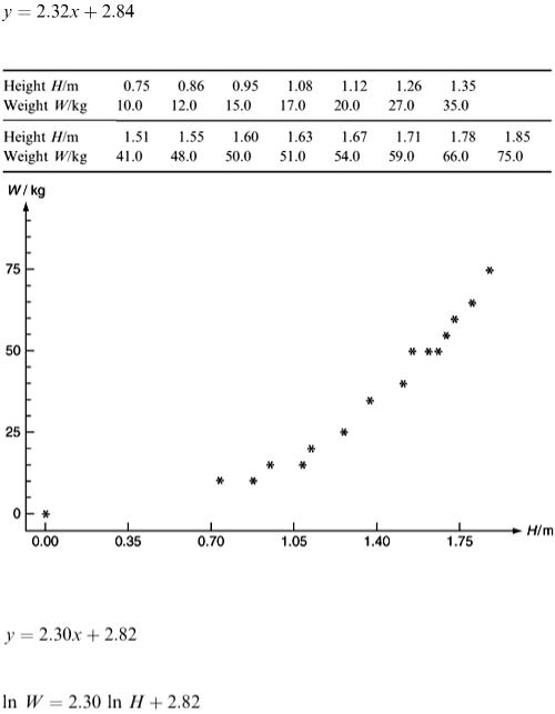
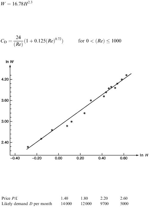
Table 8.1 records the heights and weights of a sample of 15 people of various ages. Figure 8.1 shows the result of plotting weight against height and the points seem to lie close to some curve. Note that the point (0,0) is included since zero height must imply zero weight! Both variables have been plotted as logarithms in Figure 8.2, where x = ln H and y = ln W. (This time the point W = 0, H = 0, must be left out. Why?)

The straight line fitted by eye gives

Table 8.1

Figure 8.1

Least-squares fitting of the regression model y = ax + b gives

or

So

The rather awkward exponent is typical of empirical models. As another example, the drag force on a particle of diameter d moving with speed u relative to a fluid of density ρ and viscosity μ is usually modelled by F = 0.5 C D u 2 A, where A is the cross-sectional area of the particle at right angles to the motion. The ‘drag coefficient’ C D is given by the following empirical model:

where ( Re ) = ρ ud /μ is the particle Reynolds number.

Figure 8.2

Example 8.2

Before launching a new monthly magazine the publisher carries out some market research to investigate the likely demand. This provides the following information:

What would be the best price for the magazine and what would the demand be?

The best value of P from the publisher's point of view is the one that gives the maximum revenue R = D × P. Figure 8.3 shows the graph of R as a function of P and suggests that the maximum revenue is obtained at a price of about £1.80. The peak is not very sharp, however, so it is not clear whether the best price might be £1.90 or even £2.00. A simple model can help us.

Figure 8.4 shows the graph of D as a function of P. A linear model is D = a + bP and the statistical leastsquares technique gives a = 24825 and b = −7325. At price P the demand expected is D = 24825 − 7325 P and so the revenue is R = 24825 P − 7325 P 2 . For a maximum 0 = d R /d P = 24825 − 14650 P

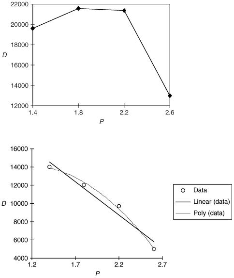
which gives P = 24825/14650 1.69. This does not seem very convincing, perhaps a non-linear model would be better. A simple model is D = a + bP + cP 2 . We use the statistical principle of least squares to find values of the parameters a, b and c giving the best fit to the data. This can be done on the Excel spreadsheet by using the SOLVER tool.

We let SOLVER find the values of a, b and c which give the minimum value of Σ( D − a − BP − cP 2 ) for the four pairs of values of D and P that we

Figure 8.3

Figure 8.4

have in the data. It gives a 8794, b 9550 and c −4219. (The same result is obtained by using Excel's Insert Trendline facility to fit a polynomial of degree two to the data.) Figure 8.5 shows the graph of the model R = P (8794 + 9550 P − 4219 P 2 ) against P from P = 1.40 to P = 2.60 and predicts a maximum R at P 1.90. (There is no virtue in finding a more precise P by solving d R /d P = 0 because a practical value of P will be a ‘round’ figure of pence.)

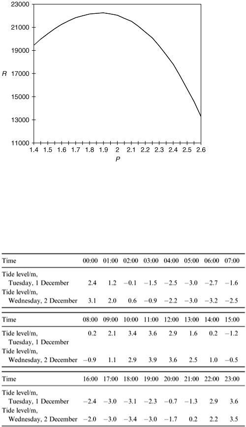
Figure 8.5

The model predicts the demand at this price to be D = 8794 + 9550 (1.9) − 4219(1.9) 2 11 700. The fit of the model to the data is shown in Figure 8.4, which also shows the linear model.

Example 8.3

Table 8.2 gives the tide level (in metres relative to a mark on a sea wall) observed over an interval of 2 days. Can we use the data to predict the tide level at 1.00 pm (13:00 hours) on Saturday, 5 December?

Table 8.2

Solution

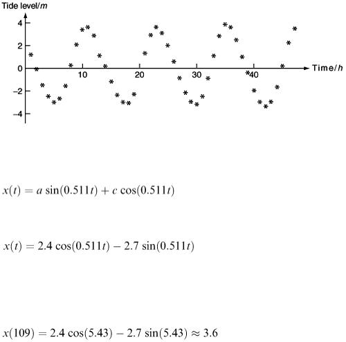
Our first step is to plot the data to get a visual impression of how the level changes with time. This is done in Figure 8.6 and it is clear that for this example a straight line or a power function is not the right kind of model. What we need is a function which repeats itself and the obvious choice is something like x = a sin( bt ). From the graph, we measure the period (time of one repetition) to be about 12.3h; so we need 2π/ b = 12.3 h so that b 0.511 h −1 .

The difference between high tide and low tide seems to be about 6.6 m, so that the amplitude is 3.3 m, but our model cannot be just x = 3.3 sin(0.511 t ) because this gives x = 0 at t = 0 (taking t = 0 to be 00:00 hours on 1 December).

Figure 8.6

We can either try to estimate the time t * when x = 0 and then use x = 3.3 sin [0.511( t − t * )] or, equivalently and more conveniently, fit a model of the form

where x (0) = c = 2.4 and x (23) = a sin(11.753) + c cos(11.753) = 3.6, so that a = −2.7. Our model is therefore

The next step would be to check the values of x given by this model for values of t from 0 to 47 against the data. However, we shall pass over this step and go on to make our prediction.

The point 1.00 pm on 5 December corresponds to t = 4 × 24 + 13 = 109 and so bt = 0.511 × 109 55.7. Subtracting multiples of 2π(8 × 2π 50.27), the answer we are looking for is

The actual value observed was 4.1; so our model's prediction was in error by 0.5/4.1 or about 12%.

Note that we have used the model to extrapolate, i.e. to make a prediction for a value of t outside the range of the data. This is a risky thing to do and it is better and safer to use a model only over the range of data from which it was derived.

Further thoughts

We notice from the graph that the mark x = 0 does not seem to be quite midway between high and low tides and that the amplitude of the oscillations seems to be increasing slightly with time. How can we modify our model to take account of these details? Would we then get a more accurate prediction?

Exercises

8.7 The following data gives the cooking time T (min) for a turkey of weight w (lb) to be cooked at

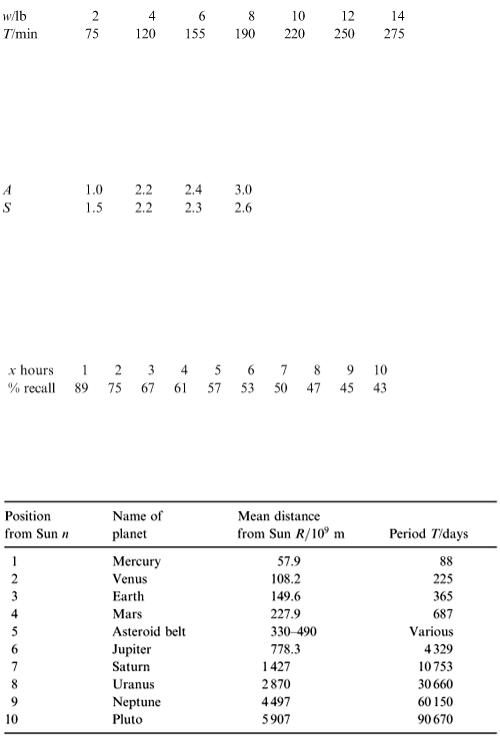
160°C.

Fit a model of the form T = aw b and use it to estimate the cooking time of a turkey weighing 8.5 lb.

A manufacturer finds that when the price of his product is fixed at £10, the level of sales S (/10 4 ) depends on the amount spent on advertising A (/£10 3 ) as follows:

8.8

Show that this can be fitted by a model of the form S = k √ A. What is the appropriate value of the constant k ?

An experimenter found that when asked to memorise a collection of objects his subject had the following percentage recall after x hours.

8.9

Find a simple model for the percentage recall as a function of x.

The following are planetary data.

8.10

1.Obtain an empirical model for finding T from R. (There is a theoretical model based on Newton's mechanics.)

2.Obtain an empirical model relating n and R.