

(Check that this satisfies the required conditions.)
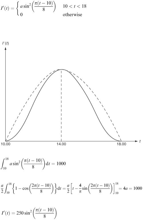
We now need to calculate the parameter a so that the total sales over the whole day amount to 1000 cones. This is easily done by integration
Figure 4.14
i.e.
So finally our model is
This means that at the height of the day at 2.00 pm we are selling at the rate of 250 cones every hour, i.e. four cones every minute.
Case 3
The jumble sale problem is somewhat different. This time we are given that 500 customers are expected; many of them will be waiting for the doors to open at the start. Suppose that the sale runs
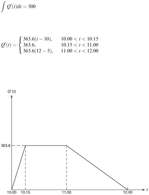
from 10.00 am until 12.00 noon. We shall need most helpers at the start to deal with the rush. Later, as many of the most sought-after items have been sold, demand will slacken off. Suppose that we are
interested in the rate of entry of customers. Denote this by Q ′( t ) where t is the time in hours. Then again, as we know the total to be 500, there is the relation
(4.1)
In Figure 4.15, we speculate on the inflow. We have indicated that Q ′( t ) is very high at the start, remains constant for the rest of the first hour and then decreases steadily to zero at the end.
As before, Q ′( t ) requires more than one equation for its specification:
The factor 363.6 is calculated from equation (4.1) above. Modelling is an activity where we want to represent trends and relations between quantities, and usually at this stage we do not want a parameter quoted to several decimal places. This means that the slightly clumsy value of 363.6 might well be replaced by 360.0, even though the customer total would then be not quite equal to 500. We do not have to use the form of Q ′( t ) just derived. You may wish to model the form in Figure 4.16.
Figure 4.15

Figure 4.16
This form suggests a mathematical representation at exp(− bt ). There are now two parameters to fix. We have the tailing off that we want, but we have to realise that Q ′ will never actually reach zero as t increases in this model. This alternative is left for you to finish, not forgetting that the time range is 10.00 < t < 12.00 and also that the integral relation holds:
Exercises
The air temperature just above the ground at a particular point on the Earth often varies in a
4.11periodic manner over a 24 h cycle. The daily mean value also varies with the seasons, i.e. over an annual cycle. If the time t is measured in hours what would be an appropriate mathematical model for the temperature as a function of t ?
In Example 2.4 (‘price war’), we assumed that the sales of both petrol stations would increase if
4.12they dropped their prices, or in other words the total petrol sales in their area would increase. Suppose instead that the local sales volume is constant so that the two garages are competing for larger shares of the same market. Suppose also
that each garage's daily sales figure is inversely proportional to the price at which they sell. Obtain mathematical expressions for each garage's daily sales in terms of their selling prices x and y.
For a certain type of tree the rate of growth is slow in winter and greatest during the summer
4.13months. The rate of growth also lessens every year from a maximum in the first year until there is virtually no growth at all after 10 years. What would be a suitable mathematical model for the rate of growth?