3.a third assistant with the same mean service times as A was employed?

7.5Using simulation models

Having developed a model which seems to simulate a system with reasonable success, do not think the major part of the work is over! A single run of the model tells you nothing more than that the model appears to be behaving as it should. To make use of the model, you need to make several runs and to analyse the results. The kind of analysis which may be needed depends on the objectives for the model and these should be stated clearly at the start. (In our hairdresser's example, our only objective was to go through the mechanics of developing a simulation model.)

In practice the objectives for a simulation model can be varied but very often they include some of the following.

1.Collecting statistics on the long-term behaviour of a system If we are trying to simulate the operation of a port, for example, we may well be interested in extremes of congestion which may occur from time to time and which will be revealed in a long-term study of the port's operation. We can, of course, run through a very long period of simulated time in a few minutes of real computing time.

2.Comparing alternative arrangements of the system This is where a good simulation model pays dividends. Making alterations to a complicated system can be very costly and time consuming in the real world. In the model world, we can make alterations quickly and easily. Examination of the results will help in deciding whether or not to go through with implementing the changes in the real world.

3.Investigating the effects of changing parameters We can use a model to find what happens if for example the mean time between arrivals decreases. Will the system be able to cope? What happens if the service times are increased?

4.

Investigating the effects of altering the modelling assumptions We may have used a rather simple model and are wondering whether it will make a significant difference if we improve it slightly.

Finding optimal operating conditions for the system There may be a number of different possible arrangements of services and queues within a system and we want to find out the ‘best’ arrangement. We shall obviously need some kind of performance measure which we can use to identify the best arrangement.

A constant problem with simulation models is the choice of initial conditions. What happens in the model depends, sometimes for a surprisingly long time, on the initial state. If we start from a rather ‘artificial’ state such as having no queues and no customers in a system, we need to run the model for some time before we get into a more typical ‘busy’ state. In many systems, this ‘typical’ behaviour, once we have reached it, carries on indefinitely and is known as the steady state. The build-up period before reaching the steady state is referred to as the transient stage.

Before running your model, consider whether you want to simulate the steady state or transient behaviour of the system. If it is the transient stage, then you must think carefully about the starting conditions. For the steady state, unless you know what a typical state of the system looks like, your only option is to put in an arbitrary set of starting values and to run the model for long enough for the effects of your starting values to be wiped out. In this case, when you come to analyse the results, you will of course ignore the data covering the transient stage. How many events you will have to generate

to reach the steady state is impossible to say; you have to experiment.

To carry out a simulation study, we make several runs of the model and collect statistics from each run. In particular, we want statistics on the performance measures mentioned earlier. Exactly what these are depends on the problem and on the point of view that we wish to adopt. From the point of view of customers the important performance measures are the following.

1.The average waiting time.

2.The average queue length.

3.The maximum queue length.

From the point of view of the system, it may be more important to look at the percentage idle time of servers and customer turn-over rate.

Note that for different runs you should use different random-number streams except when comparing two systems, when it would be useful to have exactly the same arrival pattern, for example. Note also that we talk about ‘runs’ without specifying how long each run is. Again this is something that can be decided after experimenting with your model. You can obviously

choose either of two ways of ending a run: after a specified CLOCK time has elapsed or when a certain condition is satisfied. In a model involving simple arrivals, for example, you could end the run after a specified number of arrivals.

Let us now take a more detailed look at how to collect the relevant statistics, using the hairdresser's example again. Suppose that our original objective had been to calculate the following.

1.The average waiting time of customers.

2.The average queue length.

3.The maximum queue length.

4.The percentage busy times of the two assistants.

Let us run the simulation from CLOCK = 0 to CLOCK = END. Note that there are two quite different sorts of averages involved here: an average over time and an average per customer. Let Q be the number of customers queueing at any time. The graph of Q against CLOCK time might look like Figure 7.7.

The average value of Q over time is where the total area under the graph. Let t represent an interval of time over which Q remains constant (where t itself is variable of course). As we run through the simulation, we accumulate the sum Σ( Q t ). Let N denote the total number of arrivals during the run. The two averages that we need are given by

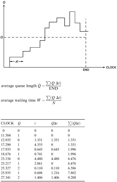
Figure 7.7

Here is part of the trace table for the hairdresser's model showing the accumulated queueing time Σ( Q t ). Note that it only shows the times at which Q changes.

The total elapsed time END is 27.341. The number N of arrivals in this time is 10. The maximum queue length Q max was 2. The accumulated queueing time is Σ( Q t ) = 9.208. The mean queue

length is 9.208/27.341 0.34. The mean waiting time is 9.208/10 0.92 min.

We ought to mention that we terminated the simulation with two customers being served — one in the queue and one newly arrived.

The total time for which server A was busy was (5 − 0) + (13.285 − 8.285) + (23.156 − 15.156) + (27.341 − 23.156) min = 22.185 min. Assistant A was therefore busy for (22.185/27.341) × 100% 81% of the time. Assistant B was busy for a total of 19.406 min or about 71% of the time.

Note that it may not be sufficient just to calculate averages because these give no indication of variability. For each run, we can give more statistical detail by means of histograms showing the distribution of waiting times, for example (i.e. how many customers waited how long). We cannot derive histograms from the Σ( Q t ) value, however, and it is necessary to record the arrival and leaving times of each customer and to store them in an array.

To give a measure of variability, we can calculate standard deviations. If we have carried out a number of runs, we can use the variation in the and values for individual runs to compute interval

estimates for the true values of and besides giving us an idea of how much reliance we can put on the results of a single run.

Exercises

The manager of a bank is considering changing over to a new single-queue system but is not sure whether it will be better for customers than the existing system. In the present system there are five service points and, when customers enter the bank, they can choose to queue at any of the five points. If a customer at the back of any queue notices that another cashier has become free, he will

7.3move over for service. The average time between the arrivals of customers in the busy period is M min and the average time taken to serve a customer is 2.5 min.

Devise a simulation model which will enable you to compare the two systems and help the bank manager to make his decision. How does the conclusion depend on the value of M ? Can you include a model for the variation in the value of M during the working day?

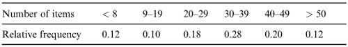
A small supermarket has four cash tills and the time taken to serve a customer at any of the tills is proportional to the number of items in his or her trolley (roughly 1 s per item). 20% of customers pay by cheque or credit card which takes 1.5 min; paying with cash takes only 0.5 min. It is proposed to make one cash till a quick-service till for customers with eight items or fewer. Two of the remaining tills are to be designated ‘cash only’.

7.4You are asked to develop a simulation model which will enable you to compare the operation of the proposed system with that of the present system. Assume that the mean time between arrivals of customers is 0.5 min and that the number of items bought by customers is represented by the following frequency table.

7.5An office has three telephone lines for incoming calls, which effectively means that a maximum of three customers can be dealt with at any one time. Customers ring at random times uniformly distributed between 9.00 am and 5.00 pm. Each call lasts for a random length of time but the average is 6 min.

The manager is worried about the possible number of customers who are unable to get through because all three lines are engaged. A certain percentage of these might try again later but some