

Figure 5.2
5.2 First-order linear difference equations
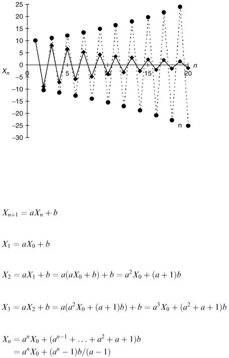
The next simplest type of difference equation is the first-order linear, constant coefficient case which we can write as:
Starting with X 0 we get
and
it follows that:
Continuing in this way
The last step comes from summing the geometric series and we have assumed that a does not equal 1. If a does equal 1 then we can see that X 2 = X 0 + 2 b, X 3 = X 0 + 3 b and so on, so in this case the solution is just X n = X 0 + nb. In the case a ≠ 1 the behaviour of X n depends on a in the same way as for the equation X n +1 = aX n except that if | a | < 1, X n approaches the value b /(1 − a ) (see Figure 5.3) either from above or from below, depending on the starting value (see Figure 5.3) while if | a | > 1, | X n | grows without limit.
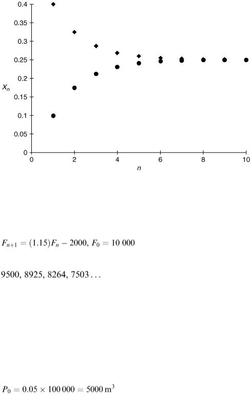
Figure 5.3
Example 5.2
A lake contains 10000 fish at present. If there was no fishing the population of fish would increase by 15% every year. It is proposed to allow fishing at the rate of 2000 fish per year. Let F n represent the number of fish n years from now. A discrete model consistent with the stated assumptions would be:
This predicts the following values for the population size in subsequent years:
On a calculator we just need to key in ×1.15 − 2000 repeatedly. On a spreadsheet after putting the first value in cell A1 we can type =1.15* A1-2000 in A2 and copy this formula down the A column. How long does it take the population to decrease to zero? The model obviously stops being usable at that point.
Suppose the lake contains 100 000 m 3 of water with 5% pollution by volume. Every day 1000 m 3 of clean water flows into the lake and 1000 m 3 of polluted lake water flows out. How long will it take for the pollution in the lake to drop to a safe level of 1%?
First note that the volume of the lake remains constant at 100 000 m 3 . We take one day as our time step and let P n represent the volume of pollutant in the lake on day n, then
and
pollution on day n + 1 = pollution on day n – outflow during day n
Each day 1000 m 3 of lake water flows out but this is partly water and partly pollution. On day zero 5% of it is pollution but as time passes this will obviously decrease. On day number n the lake contains P n m 3 of pollution inside a total of 100 000 m 3 and so every m 3 of lake water at that moment contains P
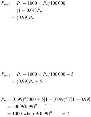
n /100 000 m 3 of pollutant and the pollution outflow is 1000 × P n /100 000. Therefore:
which means that P n = (0.99) n P 0 = (0.99) n 5000.
So P n will be down to 1000 when 1000 = (0.99) n 5000. That is (0.99) n = 1/5 or n ln(0.99) = ln(0.2), which gives n  161 days.
Suppose now that pollution continues to be added to this lake at the rate of 5 m 3 per day while 995 m 3 of clean water flows in every day and the outflow from the lake is 1000 m 3 per day. What is now our model for P n and how does this affect the answer?
We now have
This first-order linear difference equation has solution:
which gives (0.99) n = 1/9 or n ln(0.99) = − ln 9 so that n  219 days.
5.3 Tending to a limit
With some discrete models we find that as n increases the X n values are approaching a limit or equilibrium value although they never quite reach it. In this case X n +1 eventually becomes indistinguishable from X n so that X n +1 = X n = L. The value of L can therefore be found by substituting L for all the X terms in the difference equation and solving the resulting equation for L (which could be difficult). For example, if X n +1 = (5 X n − 1)/( X n + 3) then L satisfies the equation L = (5 L − 1)/( L + 3) which gives L = 1. (That was an easy one.)
In the case of the first-order linear equation X n +1 = aX n + b, if the X n values approach the limit L then, from the difference equation, L = aL + b and therefore the equilibrium value is L = b /(1 − a ) (provided we are not dealing with the case a = 1). Of course, if we happen to start with X 0 = L then we have X n = L for ever.
Example 5.3
For the model in Example 5.2 what happens to the fish population eventually? If the population size approaches a limit L then L = (1.15) L − 2000 so L  13 333 appears to be the steady-state population size. We can work out the
appropriate level of fishing F (fish y −1 ) which would keep the fish population stable at any size L from L = (1.15) L − F, that is, F = .15 L. If we had 13 333 fish in the lake we would (theoretically) always have 13 333. The fish taken out are exactly compensated by the new young fish. Apart from
practical considerations this is mathematically precarious because for one thing the right figure is actually 13 3331/3 and secondly this is not a stable population value. To see this start with a fish population just under the right figure, e.g. 13 333. Subsequently the population continues to decrease. Starting with a figure slightly over the right figure, e.g. 13 334 will give a population continuously increasing. This unstable situation is illustrated by Figure 5.4 and it occurs because the multiplication factor 1.15 is greater than 1.
Figure 5.4
Example 5.4
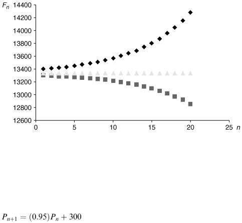
A population of herbivores living in a certain area is declining by 5% every year. As their numbers decline they leave more vegetation so more animals move into the area. Suppose this is constant at 300 animals a year, what will happen eventually?
Using P n to represent the size of the population n years from now, the model is
and the natural decline tends to be compensated by the influx of new animals. Suppose we eventually arrive at a perfect balance keeping the population size steady at a level L then L = 0.95 L + 300 so the value of L is 6000. Graphs similar to those in Figure 5.3 apply, depending whether we start below or above the
steady level of 6000. Note that the situation is opposite to that of Example 5.3, the population almost moves towards the steady value. This is because the multiplication factor 0.95 is less than 1 and the steady-state value is stable.
5.4 More than one variable
A realistic model will usually contain several variables, all probably interrelated. If they can all be modelled as discrete variables then both development with time and the relationships between variables will be modelled by difference equations. These will need to be solved simultaneously.
Example 5.5
Suppose that the water from the lake in Example 5.2 flows into a second lake containing 50 000 m 3 of water. From this second lake the daily outflow is 1200 m 3 while 200 m 3 of clean water also flows in
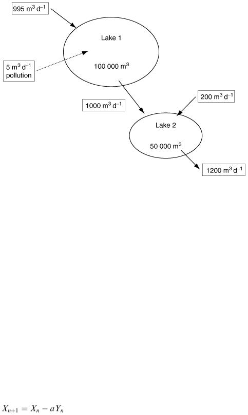
every day from a stream. Let Q n represent the pollution level (by volume) in the second lake after n days. What is the difference equation satisfied by Q n ?
Figure 5.5
The second lake receives a daily 1000 m 3 of polluted water from the first lake representing, as explained previously, a total pollution input of 0.01 P n daily. Using the same reasoning, the amount of pollution flowing out of the second lake daily is 1200 Q n /50 000 = 0.024 Q n so the modelling equation for the second lake is Q n +1 = Q n − 0.024 Q n + 0.01 P n = 0.976 Q n + 0.01 P n .
This will need to be solved simultaneously with the difference equation satisfied by P n which (in the case of a pollution input of 5 m 3 per day) was P n +1 = 0.99 P n + 5. We now have two uncoupled difference equations in that the second does not involve Q n and can be solved on its own. We can then substitute for P n into the first equation. If we are solving these equations numerically step by step, however, we do not really care whether the equations are coupled or not, the calculations are just as easy.
Example 5.6
Suppose that in a battle between two opposing forces each unit of army X is able to destroy b units of army Y during one time unit. Similarly each unit of army Y is able to destroy a units of army X.
Let X n denote the number of units of army X surviving after n time steps, and similarly Y n for army Y. We therefore have two variables and their fates are obviously linked. How does this connection appear in a mathematical model? The answer is obtained by considering what happens in one time step.
The total number of units of army X destroyed during that time step is aY n because every one of the Y n units of army Y destroys a units of army X. The number of surviving units of army X at the beginning of the next time step is therefore
and similarly for Y