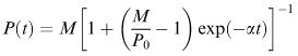
takes the form

where M = α/β and P 0 = P (0), and from this we see that the value M = α/β is never actually achieved for a finite t value. Our curves get closer and closer to the horizontal line P = M as t increases. This line represents a stable population size and various solutions arising from different initial values of P converge to it, as shown in Figure 6.2. If we had the initial value P = M, then of course we would have d P /d t = 0 for all t and the population would remain at this constant value. The population level M is sometimes referred to as the ‘carrying capacity of the environment’ and the curve is often called the ‘logistic curve’.

Exercises

A large herd of wild animals lives in a region where the rainfall varies in a periodic manner with a maximum occurring every 4 years. The animals live by grazing and the amount of food depends on

6.1the rainfall. The net birth rate can be assumed to be proportional to the amount of food available, the maximum rate being 2% per annum. There is also a net emigration of 100 animals per annum from the region. The present size of the population is 5000 animals and predictions for the next 20 years are required. Develop a model for this problem.

The rate of cooling of a hot body in air is very nearly proportional to the difference between the

6.2temperature of the body and the temperature of the air. If the temperature of the air is 18°C and a body initially at 60°C is found to have cooled to 50°C after 3 min, how long will it be before it cools to 30°C? What will its temperature be after 10 min?

A conical tank of height 2 m is full of water and the radius of the surface is 1 m. After 8 h the depth

6.3of the water is only 1.5 m. If we assume that the water evaporates at a rate proportional to the surface area exposed to the air, obtain a mathematical model for predicting the volume of water in the tank at any time t.

Assume that in the absence of fishing the population level of a species of fish would follow the

6.4same model as discussed in section 6.2. The ‘maximum sustainable yield’ Y is the maximum amount of fish biomass that can be caught annually without causing the fish stocks to decrease. Obtain a model for predicting Y from the other parameters of the problem.

6.3 Second order, one variable

No text which sets out to be a first course in mathematical modelling would be complete without some treatment of physical models involving the use of Newton's laws of motion. In a sense, in physical modelling, the ‘formulation’ part, normally a key feature in the process as described in chapter 3, is reduced as we are relying on Newton's laws to provide us with a ready-made framework on which to base the mathematical model. Close to the Earth's surface, Newton's laws are accepted as giving a reliable description of the behaviour of mechanical systems. We have certainly no intention of challenging Newton here; so it appears as if the student modeller is in for an easy time! If this were completely true, it would be a pity since it is usually the formulation stage which gives the greatest challenge, i.e. you have the opportunity of building up relations and equations between variables based on your own assumptions or collected data.

In considering a model for a physical or mechanical system, we shall be seeking an equation of motion based on Newton's second law. We do not attempt to interfere with this law; however, it often turns out that not all the constituent parts of the equation of motion will be beyond discussion. For example, any situation involving consideration of air resistance, frictional effects, size of moving object, etc., will need our modelling judgement as to their inclusion in the model.

While we are discussing preliminaries, it is important to point out that mathematical modelling and models are common in the ‘real’ world where there is a physical or engineering system under investigation. It is not a question of tinkering with problems found in textbooks on classical mechanics. Modelling a physical system is widely carried out in industries involving the transportation or flow of a substance: gas, coal, steel, electricity, nuclear power, etc. Also the modelling of wave behaviour is important in radar and submarine detection work.

In section 6.2, we looked at a model for population growth and this will be followed in section 6.5 with a harder population model and also a battle model. These could be classified as biological models, although it can be a mistake to classify too rigidly. A physical systems model is intended to refer to situations involving physics such as mechanics, heat transfer, sound waves and electricity. Thus we are concerned with dropping, swinging, throwing, hitting, heating and cooling, flowing, diffusing and possibly even permeating.

As we have already said, the development of models for physical systems relies very heavily on the application of Newton's second law of motion. This can be stated as follows:

(assuming constant mass).

Now this section deals with second-order differential equations, and it is the concept of acceleration which gives us the second derivative term. We shall not describe here the full details of theoretical mechanics since there are many good texts on the subject (see, for example, the book by Medley listed in the Bibliography). Instead we concentrate on the creative theme embodied in modelling. Two examples will now be investigated which contain this theme. In both of the resulting models, we shall find that the mathematical representation results in a second-order differential equation, and this contrasts with the models in section 6.2 which all resulted in first-order differential equations. Also both examples contain aspects of mechanics that are found in first-course modelling books, but the examples also contain interesting features which you may not have met before.

Example 6.2

This example is set in the context of a recent case in the court of appeal. The client was a convicted murderer suspected of having jumped from a high window to avoid detection for burglary. The legal problem centred on the client's claim that, had he been the person jumping, then he would have severely injured himself owing to previously known personal leg joint weakness. The mathematical problem was to estimate the impact speed in these circumstances to see whether it was likely that the person could then get up and run away!

Problem statement

The particular question posed was ‘If someone fell a distance of about 30 ft, what would the impact speed be?’

Formulate a mathematical model

Here is our chance to make some modelling judgement about the nature of falling human bodies: is it

free fall or air-resisted fall? Does the size of the falling body matter in this case? Assuming that air resistance does have an important effect, how are we going to assess it in our model? Following our usual procedure we first list the factors involved (Table 6.1).

Now there are useful general connections between x, v, t and f using differential calculus which can be applied in this context:

Table 6.1

Note that, for convenience, d x /d t and d 2 x /d t 2 are written as and respectively. Also

A diagram usually helps in situations such as this; so, before applying Newton's second law, we shall give one, labelling it using the above notation (Figure 6.3). Note that O is the point from which the body starts its motion and the variable x denotes the distance fallen vertically downwards in time t. All mechanics problems need a fixed frame of reference and, as the motion is vertically downwards, we have a one-dimensional problem.

The forces acting have magnitudes mg and R in the directions shown on the diagram; so the net external force on the body has magnitude mg – R. Applying Newton's law (in a downward positive sense), we get

This is our model. It is not completely formulated as R has to be specified. Note also the mg term at the beginning of the equation, which represents the force due to gravity. The acceleration due to gravity can be measured experimentally in vacuum to be constant near the Earth's surface. This constant value is approximately 9.8065 m s −2 or 32.2 ft s −2 . Thus,

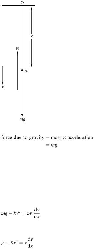
Figure 6.3

To proceed further, we need an expression for R. Air drag is a common enough experience whether running, cycling or even walking. (Is it the same thing as considering the effect of the wind?) A moment's thought tells us that R will not be distance or time dependent (why not?) but will be velocity dependent, i.e. the faster you go the greater the air drag. So we model air resistance as R = kv, provided that R is directly proportional to v.

Suppose that a more complicated relation is proposed, such as R = kv 2 or, more generally, R = kv n . How are we to know which is the best model? The answer to this is that it depends what sort of object is being dragged. For the moment, let us take the general relation R = kv n , and the equation of motion then becomes

We can divide through by m, redefine the constant of proportionality k as K = k / m and so produce a neat mathematical model:

However, what is to be done about the index n? A number of attempts have been made to decide this, and also the value of K which now contains dependence on the mass m of the object. These decisions are important in modelling; so we must not fudge the issue. We shall use the following information

from books on mechanics.

1.For a small compact object such as a stone, air resistance is directly proportional to speed, i.e. n = 1.

2.For large bulky objects such as a human body, air resistance is directly proportional to the square of the speed, i.e. n = 2, and this is what we shall use in our model. This makes the mathematical model easier to solve than if n were taken to be, say, 1.347.

The value of K has also to be worked out so that the magnitude of the air resistance can be correctly estimated. This can be done by looking up a text-book on mechanics or, better still, using the concept of ‘terminal speed’. The terminal speed is the ultimate constant speed acquired by a body moving freely in a medium such as air. It is reported that the terminal speed of a human is about 120 miles h −1

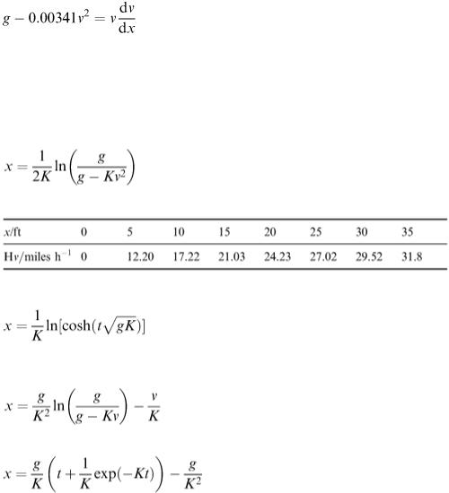
. In this situation, there is no acceleration (gravitational pull balances air resistance) and from the differential equation this means that g – Kv 2 = 0. Converting 120 miles h −1 to the equivalent value in metres per second and substituting g = 9.8065 gives K = 0.00341. Thus, our model for the motion of a body falling out of a window is represented by the first-order differential equation

Obtain the mathematical solution

Provided that n = 2 (as here) or n = 1 the equation can be integrated directly. It does not worry the modeller, however, to be told that n = 1.347 since numerical methods can be used or perhaps a simulation package which deals with general differential equation models. The mathematical solution for n = 2 is

(6.2)

Table 6.2

If we want the relation between distance fallen and time elapsed, then further integrations give (6.3)

( K = 0.00341). The corresponding results for the dropping of a stone (where n = 1, and a different K value is then needed) are

(6.4)

and

(6.5)

Equation (6.2) can be used to tabulate x and v. The original question about the man jumping out of a window can now be answered. We must convert the units to feet and miles per hour since that is how the appeal court will want them. Using the conversion factors from chapter 4, Table 6.2 can be drawn

up.

The particular distance jumped or fallen was said to be 30 ft; so the model predicts that the speed on hitting the ground is 29.52 miles h −1 .

Interpret the mathematical solution

First note that to declare a value for the impact speed correct to two decimal places is not sensible for the following reasons.

1.The precise distance dropped is not known, only ‘about 30 ft’.

2.The result is best given correct to the nearest whole number for simplicity.

The advice produced from our model is that, if you fall about 30 ft, you hit the ground at about 30 miles h −1 . This could be compared with being in a car crash at 30 miles h −1 ; so we expect some injury. Also, in parachute

training, instructors often say that the impact will be like falling off a 12 ft wall, which from Table 6.2 is equivalent to an impact speed of 19 miles h −1 .

It therefore seems reasonable to suggest that falling 30 ft would give some injury, the impact speed being about 50% higher than that for a parachutist. However, this does not take into account the nature of the ground where the landing takes place. Perhaps a soft landing in a flower bed might allow the burglar to get away unhurt. Can we include these considerations in our model?

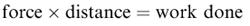
Injury on impact will be related to the magnitude of the average force experienced on hitting the ground. We can make a numerical estimate of this using the principle that

In this case the force concerned will be the average force experienced over the time interval during which the person is sinking into the soil and the distance will be the depth to which he sinks. The work done is equated to the total kinetic energy on impact, given by 0.5 × mass × (speed) 2 . Knowing the mass and speed, if we also know the depth of sinking into the soil, we can calculate the average force experienced. Our advice to the court is to examine the ground below the window.

Further thoughts

1.If air resistance is neglected, what difference does this make to the model and what answer is then obtained?

2.If examination of the soil beneath the window reveals footprints 10 cm deep, what can we deduce?

Example 6.3

You will probably be familiar with the model for a simple pendulum. Here we shall deal with a more interesting real-life situation. Suppose that a heavy mass is being swung against on old high wall on a demolition site. The situation is quite common where old buildings are being knocked down prior to site redevelopment. The heavy mass is supported from the end of a crane cable and is made to swing by the crane driver making the crane jib move backwards and forwards. The objective is to make the mass strike the wall as hard as possible so that parts of the wall fall down. The crane driver can also pay in or pay out the cable as the mass is swinging backwards and forwards.

Problem statement

A single wall of height 12 m is to be demolished. The crane jib is 15 m above ground level and the

perpendicular to the wall when activated by the driver. As its movement will be relatively small compared with the height of the wall, this seems a reasonable approximation. This means that the cable AP will move in a vertical plane perpendicular to the wall. Thus, from the diagram, BD, OD and ON are fixed lines.

The mathematical model will be based on applying Newton's second law to describe the motion of the mass P. This requires the acceleration of P to be expressed in terms of the problem variables x, r and θ. With respect to the point A, P has polar coordinates ( r, θ). The radial and transverse components of velocity and acceleration in terms of polar coordinates are well known (see, for example, D. G. Medley, An Introduction to Mechanics and Modelling, Heinemann, 1982). Let us mark them on a separate diagram (Figure 6.5) for easy reference.

As the point A is itself moving horizontally with displacement denoted by x, then an additional horizontal acceleration component is added. This is shown in Figure 6.4. There will be two forces acting on P, again labelled in Figure 6.4. These are the gravity force mg and the tension in the cable denoted by T. (We assume calm local conditions; so wind and air resistance are neglected.)

In order to knock down the wall, we imagine the crane driver causing the jib arm to move back and forth so that oscillations are transferred to the point P. In two dimensions, when Newton's second law is applied, we can expect two equations of motion, but a moment's thought tells us that we are not really interested in bringing into the mathematical model the value of the cable tension. Consequently consider the equation of motion in a direction perpendicular to the cable. The resulting acceleration component in this direction will be

made up from the polar terms relative to A, together with the term from the motion of A resolved in the direction perpendicular to the cable. The equation of motion is

(6.6)

As expected, this is a second-order differential equation in the variable θ but also containing the variables x and r. However, these can be considered as inputs to the model as they are under the control of the driver.

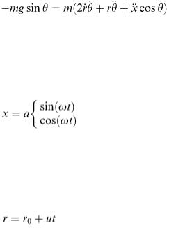
Now the crane driver has to activate the system by swinging the jib backwards and forwards. This can be modelled by taking the variable x to have a periodic form of the type

(6.7)

according to the starting conditions that we select. This function is an obvious choice for representing the physical effect that we are seeking. By suitably choosing values for the amplitude a and the frequency ω, we can model the desired effect.

We now consider the pay-out of the cable. We might suppose that the initial length of the cable is a certain value, say r 0 , and, if we pay out the cable at a steady rate u, then a model for the variable r is

(6.8)

By substituting from equations (6.7) and (6.8) for x, r and their derivatives the differential equation for θ is

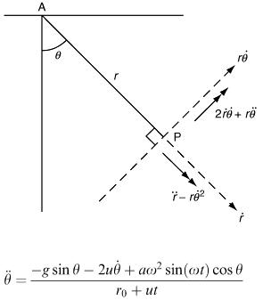
Figure 6.5

(6.9)

Note that other forms of equation (6.9) will be obtained if alternative models are used for x and r. For example using equation (6.8) means that the pay-out speed of the cable is always u which is counter to the original condition that the mass at P is initially at rest.

Equation (6.9) is considerably more complicated than the one we had in Example 6.2. We could decide to simplify the model, but in any case the mathematical solution will probably require a numerical method or perhaps the use of a simulation package.

Another interesting factor here is that, by solving the above equation, we shall not exactly provide information that a crane driver can use or indeed is actually interested in. He is concerned with where to position his crane and also what speeds can be generated by the swings that he is setting up.

This is an example where the mathematical results obtained from a difficult differential equation, although interesting in themselves, are not the primary concern of the mathematical model. The questions of the speed of the mass and the position of the crane can be dealt with by returning to the diagram and considering the relevant variables. A new diagram (Figure 6.6) showing the velocity

components is helpful. (Note that and are components of P's velocity relative to the point A.)

The position of the mass with respect to the coordinate origin O can be easily worked out from MP and OM:

Figure 6.6

We are interested in the speed with which the mass hits the wall. More particularly, since damage is to be inflicted by the blow, it is the horizontal velocity component that has to be calculated, given by

Obtain the mathematical solution

We are now ready to investigate the solution of the mathematical model. We must decide where to start the jib oscillations from, and what energy to put into the system. We also have to consider whether to pay out the cable and at what rate. Most importantly of all, we have to know the dimensions of the wall to be demolished and how close to this wall we can position the base of the crane. This means that the parameters a, u and ω have to be chosen.

To take a particular case, we shall use the following data, but you may like to try other values: a = 3.0 m, u = 0.3 m s −1 , ω = 1.0 s −1 and r 0 = 8.0 m. Initially P hangs below the point D (see Figure 6.6).

Interpret the mathematical solution

With the above data, we find that the wall will be struck after one swing with a speed whose horizontal component is 9.0 m s −1 at a height of about 11 m. There is a final comment to make about the use of this model, and that is that the wall will be knocked down according to the size of the blow inflicted. The value of the mass m has not been needed so far, but the magnitude of the blow will be given by the horizontal momentum at impact, i.e. m × v horiz. We also do not know the strength of the wall, but we assume it to be only so strong that this method of demolition is suitable.

Exercises

6.5Newton's laws: fact or fiction exercises Often when we come to apply Newton's laws in mathematical models, the first problem is to be sure that we have understood the mechanical principles involved. If your modelling has been supported by, say, a parallel course in dynamics and statics or some suitable alternative, then you will probably have no trouble in marking in the correct

forces and accelerations in a given

physical situation. If you are more uncertain, try the following exercises. Classify the following as true or false.

1.A force always produces motion.

2.A body always moves in the same direction as the force acting on it.

3.If no force is acting on a body, then the body must be at rest.

4.The velocity produced in a moving body is directly proportional to the force acting.

5.When a ball is thrown vertically upwards (Figure 6.7), then at A (the highest point reached), the velocity and acceleration are

1.both zero

2.one of them is zero (which?), or

3.neither is zero.

6.When a ball is thrown as a projectile (Figure 6.8), then at B (the highest point)

1.the horizontal velocity component is zero,

2.the horizontal acceleration component is zero,

3.the vertical velocity is zero, or

4.the vertical acceleration is zero.

6.6Now try to answer the following problems.

1.When you push a door shut, why is it easier to push near to the door handle than near to the hinge?

2.Why is it easier to pull a heavy object (i.e. a lawn mower or a sledge) along than to push it?

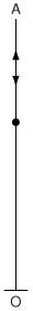
Figure 6.7

Figure 6.8

How does the fairground wall of death work? Why do astronauts experience weightlessness in a capsule a few hundred miles up from the Earth? 6.7 On some ‘private’ estates and also within the grounds of a hospital, the authorities install a series of small ramps across the road to prevent motorists from exceeding a certain speed limit. (The ramps are sometimes called ‘sleeping policemen’!) The effect of driving too fast over such a ramp will be to cause the driver some discomfort and he or she may hit the car roof. Investigate the situation when a car moves over the ramp. Consider the effect of the springs of the vehicle which is travelling over a flat road. The springs will be compressed into some steady-state condition. A car suspension system also uses dampers to prevent continuing oscillation. Using the very simple model of a car shown in Figure 6.9, formulate a differential equation for the displacement of the driver. This will be a second-order equation and is not too difficult to solve. (You will need to use Hooke's law to model the car spring: the force of tension or compression is directly proportional to the amount that the spring is stretched or compressed. Also assume the damper force is proportional to the rate of change of displacement.) The data are as follows: the mass of the car is 1000 kg, the spring stiffness is 5 × 104 N m−1, the damper coefficient is 9 × 104 N m−1, and the ramp is about 1 m across and its height is about 30 cm. 6.8 A common feature of all public buildings is some mechanical device which will automatically close a door after someone has passed through. Can you set up a model to explain how the effect is usually for the door to close fast when swung wide open, but to close more gently as it moves to the shut position? This seems quite a large task,

Figure 6.9

and so we shall suggest two systems for investigation: one simple (case A) and the other more complicated (case B).

Case A is depicted in Figure 6.10 which shows a simple ‘arm’ which presses onto the door with a certain force due to a coiled spring in the spring unit. The idea is that, with the door almost shut, the pressure from the arm has reduced almost to zero. As far as the motion of the door is concerned, you will need to regard its motion as that of a rigid body. This means that we shall need to know the ‘moment of inertia’ of the door about the vertical hinge axis (see, the book by Medley listed in the Bibliography).

Case B is the more common two-armed version shown in Figure 6.11. Here contact between the mechanism and the door and door frame are at fixed places and there are two freely joined arms which cause the door to close.

Figure 6.10