

4.7 Relative sizes of terms
A model will often combine together a large number of variables, some with more effect than others on the final result. There is no point in including in the model more variables than are necessary to give an answer with the required amount of accuracy. If a particular variable makes an insignificant contribution to the answer when compared with the contributions of other variables, then it makes sense to abandon that variable especially if this simplifies the model. The same principles apply to expressions and equations which appear in the model. If an expression or equation involves a number of terms, it is often instructive to calculate roughly the relative sizes of the terms. Dropping the least significant terms will often simplify the mathematics considerably with no serious effect on the accuracy of the model.
Suppose that a variable x is known to have a value around 10. We use the notation x  O (10) to mean ‘ x is of the order of 10’ or ‘ x is in tens rather than in hundreds’. We have 1/ x = x −1
  O(10 −1 ) and x
2  O(10 2 ) so that in the expression y = 1/ x + x 2 we have a sum of two terms whose magnitudes are O(10 −1 ) and O(10 2 ). The second term is three orders of magnitude (a factor of 10 3 ) larger than the first; so, if we replace the original expression by y = x 2 , the relative error that we are making (see section 8.4) should be about 10 −3 . For example, suppose that x = 8; then 1/ x + x 2 = 64.125, while x 2 = 64 and the relative error is 0.125/64
  0.002. If the original expression had been
we could replace it by the considerably simpler version
without much loss of accuracy.
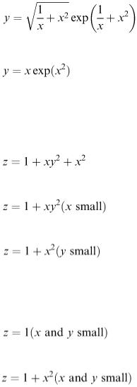
In experiments containing several variables and parameters, we must evaluate the order of magnitude of each term. Generally the approximation that we get depends on which variable is smallest and it is sometimes useful to indicate this using a notation such as ( x small). For example, if
then we can say that
and
In each case we have dropped squares (and higher powers if there had been any) of the variables concerned. Consequently what we have obtained are referred to as ‘first-order approximations’. Second-order approximations are obtained by dropping powers higher than second. In the above example, if both x and y are small, then
is the first-order approximation and
is the second-order approximation for z.
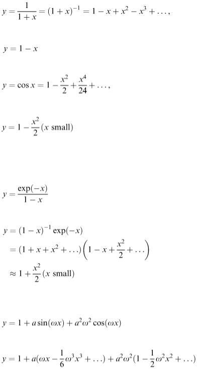
Series expansions such as Maclaurin series are useful for obtaining low-order approximations. For example, if
we can write
to first order in x. Similarly, if
then
This is a second-order aproximation.
Example 4.6
If
we can write
Example 4.7
If
then
So
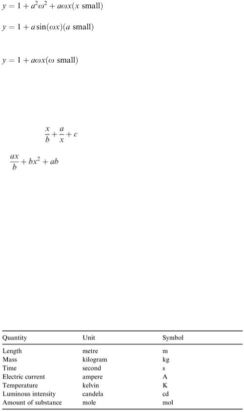
and
Exercises
In the following questions the parameters a, b and c have the values a = 0.1, b = 0.01, c = 0.001 and the variable x can be assumed to lie in the interval [1, 10].
Identify the smallest and the largest terms in each of the following expressions.
4.14
1.
4.15 Simplify the following expressions by rejecting the smallest term in each. 4.16 Simplify the following by rejecting all terms of order 10−n with n > 2. 4.17 Simplify the following as far as possible by retaining only the largest terms.
4.8 Units
There are several different systems of units which have been used in the past and unfortunately are still in use today. We therefore need to be clear about which particular system we are using and keep to it consistently. It will often be necessary to convert from one system to another. We may find that the data we need are in the ‘wrong’ units and we need to know the relevant conversion factors. Most of the examples in chapter 2 involved units (Examples 2.4, 2.6 and 2.11) and some (Example 2.3) involved a mixture of units.
The recommended scientific system of units is the SI system (short for Système International d'Unités). This has seven basic units with accepted symbols as shown in Table 4.2.
Table 4.2
There are also other commonly used units which are combinations of some of these and have been given their own names and symbols – see Table 4.3.
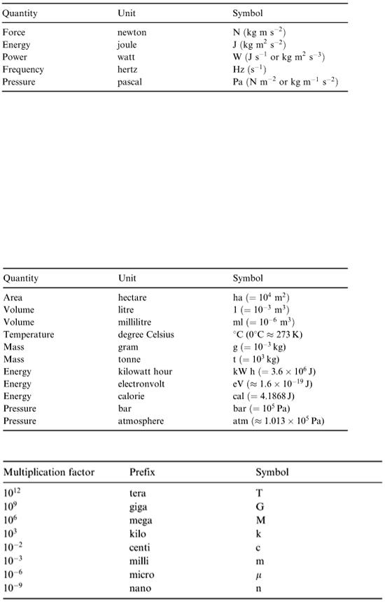
Table 4.3
Note the use of both positive and negative indices where a combination of units is involved. Speed, for example, is measured in metres per second which in this book is abbreviated to m s −1 (the alternative m/s is sometimes used in other work). Similarly, for acceleration (which is measured in metres per second per second), we use m s −2 rather than m/s 2 (m/s/s should not be used at all).
There are a number of non-SI units which are in common use by scientists and engineers. The main ones are as shown in Table 4.4.
In the real world, there is such a wide range of sizes for all sorts of quantities, it is inevitable that the seven basic SI units are inadequate in their basic form. So we use special symbols for large and small multiples of the basic units. These are based on powers of 10 and the names and symbols shown in Table 4.5 are the prefixes most commonly used.
Table 4.4
Table 4.5
For example, the power output of a generator will often be measured in megawatts (MW), building measurements are often in millimetres (mm) and computer operating times are in nanoseconds (ns).
Angles are measured in radians (symbol, rad). 1 rad is the angle between two radii of a circle which cut off on the circumference an arc equal to the radius. In three dimensions, solid angles are measured in steradians (symbol, sr). Other units for angles are the degree (symbol, °) which equals π / 180 rad, the minute of arc (symbol, ′) which is (1/60)° or π/10 800 rad, and the second of arc (symbol, ′′) which is (1/60)′ or π/648 000 rad. Conversely, 1 rad  57.295°.
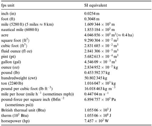
Another system of units which is still in use is the British or foot–pound–second (fps) system. The main units and their conversion factors are given in Table 4.6. (Use reciprocals to convert the other way.)
The continuing use of the Fahrenheit scale of temperature can be a nuisance. To convert from °F to °C use °C = 5(°F − 32)/9; conversely, °F = 9 × °C/5 + 32.
Table 4.6
Note that the above tables show the recommended usage regarding abbreviations and symbols but it would be misleading to pretend that these are strictly adhered to in real life. In modelling, we can expect to come across data measured in a variety of units often mixed up together as well as different abbreviations and symbols for the same units. It is common, for example, to see in and ins for inches and s or sec or secs for seconds. ISO recommendations have been used in this book, i.e. in for inches, and s for seconds.
Example 4.8
A girl who has a mass of 8 stones eats a 50 g bar of chocolate. The energy content of the chocolate is 4700 kcal kg −1 . Assuming that her digestive system is able to convert all the chocolate bar's energy