into the model? What are the results?

7.In reality there must be a time delay before a large surplus of food results in an increased number of baby foxes. How can we include this? What effect does it have?

In Example 6.7 we took both c 1 (0) and c 2 (0) to be zero but in Example 5.5 c 1 (0) was not zero but 5000/100 000 = 0.05. What difference does this make to the model?

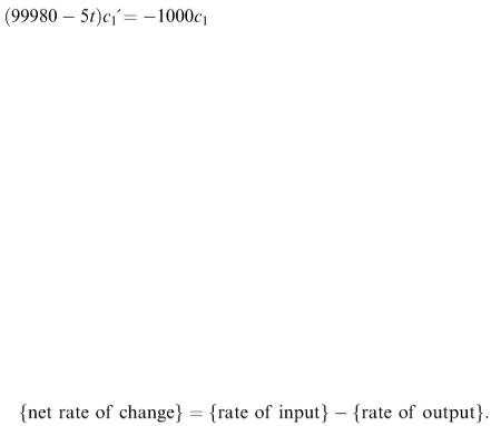
Suppose that the input of pollution to Lake 1 continues at the rate of 5 m 3 per day for four days and then stops. For time t > 4 the volume of Lake 1 will now be 100 000 − 5( t − 4) so the

6.17 differential equation for c 1 changes to

Show that this predicts a maximum pollution of about 1123 m 3 in Lake 2 after about 64 days.

Summary

In this chapter, we have looked at some models involving differential equations. This is a very important area of mathematical modelling since very many models involve variables changing with time. As with all modelling problems, there is no standard method of setting up the differential equations relevant to the particular problem in hand but the following points may be useful.

1.After writing down the problem statement and listing your assumptions carefully, read through and look for the words ‘change’, ‘rate’, ‘increase’, ‘decrease’, ‘growth’ and ‘decay’. Any of these words will usually imply that a differential equation may be appropriate.

2.Differential equations result from applying an assumption or a ‘law’ governing rates of change. Is there a well-known scientific law which applies to your particular problem (such as Newton's mechanics) or do you have to derive one from your own assumptions? Very often the relevant differential equation will come out of the following very simple ‘input-output’ principle:

Although this seems very obvious, you will find in practice that, once you have written this down and substituted appropriate expressions involving the variables which appear in your model, you will have your differential equation in front of you.

3.Before rushing into trying to solve a differential equation, stop to think. Does the equation make sense in terms of what you know about how the

model should behave? Check that each term in the equation has the same physical dimensions (see chapter 4). If time is the independent variable, the choice of time unit is up to you; it could be seconds, hours or years.

Choose whatever is most appropriate for the time scale of the model that you are dealing with. Make sure that any parameters, etc., that appear have values referred to the same time unit. Can you draw any conclusions from the equation without solving it? Are there any values of the variables for which the derivative is zero? What are the implications? Under what conditions are the derivatives positive, negative, very large and very small? Does the equation imply any restrictions on the values of the

variables, e.g. the equation is meaningless if x < 5. Are there any restrictions on the variables arising from physical factors?

Solve the equation analytically if the integration looks easy. Remember that a single integration of a first-order differential equation will give you a set of solution curves with an arbitrary constant. Use any available particular information such as starting values of the variables to derive the values of arbitrary constants. If an analytic solution seems difficult to obtain, use numerical methods. There are many methods to choose from and also software packages for both large and small computers are available, especially designed for modelling problems involving differential equations.

CHAPTER 7

Using Random Numbers

Aims and objectives

In this chapter we develop models in which one or more variables are modelled as random. We look at how such models can be implemented in practice using computer-generated random numbers.

7.1 Introduction

In chapter 2, we came across situations where chance played a part and some of the variables were random variables. In chapter 3, we described models involving random variables as ‘stochastic’ or ‘probabilistic’ models. They obviously form a very important class of problem since uncertainty is an ever-present feature of real life. Here we look a little more closely at what is involved in developing and using probabilistic models.

7.2 Modelling random variables

What exactly do we mean by a random variable? Clearly a random variable is one whose value is unpredictable in advance, but there is more to it than that. Although an individual measurement of a random variable is unpredictable (except possibly to say that the measured value cannot fall outside a certain range) the long-term pattern of values is predictable in a statistical sense. We take the view that randomness is not chaos but has a pattern to it and it is this pattern of randomness that we try to model.

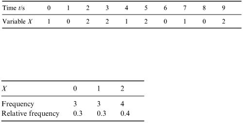
Can we find a model for the following data?

X appears to be a discrete random variable taking the values 0, 1 and 2. It is not possible to write down a deterministic formula relating X and t. Instead, we

describe the pattern of randomness mathematically by counting the number of times that the different values of X occur and putting together a frequency table as follows.

This table gives us the pattern for the random variable X. The relative frequencies tell us what percentages of the measurements of X have resulted in that particular value. If we needed to build a model involving this random variable, we could assume that this pattern will always apply no matter how many times we measure X. We would be making a general assumption based on very few data and in effect treating the relative frequency distribution as a probability function. An alternative would be to assume a simple theoretical model for the probability function. For example, we could assume that the three values are in principle equally likely so that the probability function is as follows.

This example illustrates the two choices that we have in creating models for random variables.

1.Use a theoretical model. In any book on mathematical statistics, you will find several standard theoretical models such as the binomial distribution and we shall discuss the main ones later. Each one is based on certain assumptions holding true; so our choice depends on making the appropriate assumptions for our particular model.

2.Use the relative frequency table based on actual data without attempting to fit a standard theoretical model.

The advantage of the first approach is that we can make exact statements about the probabilities of various outcomes and we have the power of mathematical statistics at our disposal. This advantage, however, is limited to fairly simple situations. As the complexity increases, the mathematics becomes too difficult. The advantage of the second approach is that we are conforming exactly to observed data rather than using models based on assumptions, and increasing complexity does not present a great problem, simply more work. The disadvantage is that we are no longer able to use mathematical analysis and instead we have to resort to simulations and to rely on statistical results from our models.

When making our choice of model, the first important consideration is whether we are dealing with a discrete or a continuous random variable. A discrete random variable is one that can take any value from a set of distinct values but nothing in between. For example the number of children in a family has to be a non-negative integer. A continuous random variable, on the other hand, can take any value within a certain range, e.g. a child's height. In practice the distinction between the two types is often blurred because continuous variables will be measured to the nearest unit on some scale of measurement, e.g. height to the nearest centimetre. One of the modelling decisions that we may have to make is whether to represent a particular variable as continuous or discrete.

Theoretical models for discrete random variables are specified by a probability function p ( x ) = Prob( X = x ), which is the probability that the random variable X takes the value x. The simplest model is the discrete uniform distribution where each value has the same probability. This is what we would probably use if X represented the score on an ordinary six-sided die as used in games of chance.

A very useful discrete model is the binomial distribution. If there are n independent items, each of which has a constant probability p of being a certain type, then the number X of items of that type is a random variable whose probability function is

Suppose that events occur at random such that in a small time interval t the probability that an event occurs is λΔ t and the probability that more than one event occurs is zero. If X is the number of events occurring in one unit of time, X is a random variable whose probability function is

This is the Poisson distribution and the sequence of events is described as a Poisson process.

Data on a discrete random variable can be put into a relative frequency table as we did for the first

example in this section. When the number of observations is large, we expect the relative frequencies to correspond closely to the values of the probability function.

Theoretical models for a continuous random variable are specified by a probability density function (pdf) f ( x ) where f ( x )≥0 for all x and 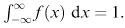The probability that the random variable takes a value between x 1 and x 2 is given by

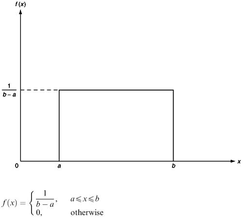
The simplest example is the continuous uniform distribution on the interval [ a, b ] (Figure 7.1). For this,

Figure 7.1

For example, if θ is the angle that a spinning pointer makes with a fixed direction when it finally comes to rest, then (unless the pointer has a tendency to stick in a particular direction) θ is a random variable and the appropriate model is the continuous uniform distribution on [0°, 360°].

In the Poisson process described earlier, the time gap between consecutive events is obviously a continuous random variable. Its pdf is f ( x ) = λexp(−λ x ), x ≥0, and it is known as the exponential distribution (Figure 7.2).

Note that small time gaps are quite common (high probability) while long time gaps are rare. The mean time gap is 1/λ.

Another very useful and popular model for continuous random variables is the Normal distribution (Figure 7.3). The pdf is

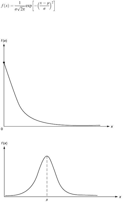
There are two parameters μ and σ; μ is the mean and determines the central position while σ is the standard deviation and determines the ‘width’ of the curve.

Data on a continuous random variable can be put into a relative frequency table just as in the case of a discrete random variable but the difference is that in

Figure 7.2

Figure 7.3

the case of a discrete random variable each relative frequency corresponds to a particular value of the random variable. For a continuous random variable, each relative frequency corresponds to a range of values of the random variable. For example a student finds that his journey to college can take up to 20