9.5 Disk pressing

Context

You are employed to give advice to the production manager of a manufacturing firm. Part of the production process requires the cutting of circular disks from 1 m × 1 m sheets of steel. At present the disk-pressing machine is set to press out 16 disks of diameter 0.25 m from each sheet. You are asked whether it is possible to rearrange the cutting heads to save on wastage. There is also a need to cut disks of diameter 0.1 m from the same sheets. What would be the best arrangement of the cutting heads to minimise wastage? Is it possible to produce a mathematical formula for the maximum number of disks of radius r that can be cut from a sheet of given dimensions?

Problem statement

Given the size of disk and the dimensions of the sheet, find the most efficient cutting pattern and the maximum number of disks that can be cut from one sheet.

Formulate a mathematical model

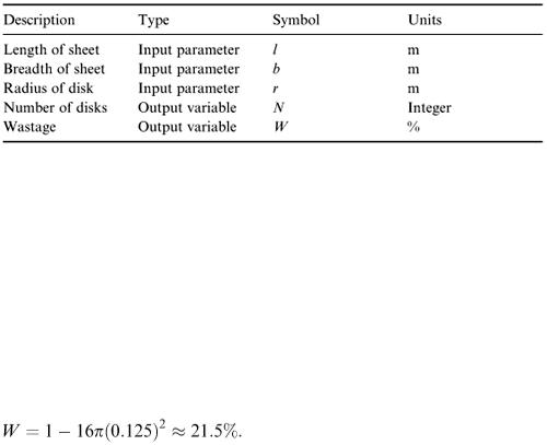
We can list our factors as in Table 9.7.

Table 9.7

Assumptions

1.The disk cutters can cut cleanly and with perfect accuracy so that we can let the circles touch on our diagrams.

2.We shall examine patterns in which each circle (except those near an edge) touches

1.four others (‘four-point contact’ or ‘square arrangement’) and

2.six others (‘six-point contact’ or ‘triangular arrangement’).

Obtain the mathematical solution

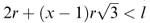
The simplest pattern is the square arrangement with four-point contact as shown in Figure 9.5. For the case mentioned above, we have l = b = 1, r = 0.125 and N = 16; so the wastage is

If the same pattern is used for the case l = b = 1, r = 0.05, then N = 100 and W = 1 − 100π(0.05) 2 21.5% as before. (Is this surprising?)

For general values of the parameters, we can form n columns of disks with this pattern if b > 2 nr (Figure 9.6). If we increase b, another column becomes possible if b reaches (2 n + 2) r. This means

that n is the integer part of b /2 r which we write as [ b /2 r ], the square brackets denoting ‘the integer part of’. An exactly similar argument applies to the rows, from which we deduce that the

Figure 9.5

Figure 9.6

number of rows is [ l /2 r ]; so the total number of disks is N = [ b /2 r ][ l /2 r ] and the wastage is W = ( lb − [ b /2 r ][ l /2 r ]π r 2 )/ lb.

Let us now look at the possibilities with six-point contact and general values of l, b and r. If we think of the pattern in terms of horizontal rows, it is clear from Figure 9.7 that, when b is an odd-integer multiple of r (i.e. (2 n + 1) r ), then each row can hold n disks and, if b is increased, this remains true until b reaches (2 n + 2) r when an extra disk can be fitted in alternate rows. At this stage, we have alternate rows of n + 1 and n disks. If b is increased further, the same pattern applies until we reach b = (2 n + 3) r when equal rows of n + 1 disks become possible.

Figure 9.7

Looking down the vertical side in Figure 9.7, we see that, if there are x rows, then

and, since x must be an integer, we can write 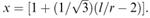In the case of equal rows of n disks the total number of disks is N = nx and, since we have the condition (2 n + 1) r ≤ b < (2 n + 2) r, we can write down the value of n as

So

In the case of unequal rows of alternate n + 1 and n disks the number of long rows (each with n + 1 disks) is x /2 if x is even, and ( x + 1)/2 if x is odd. Also n has to satisfy (2 n + 2) r ≤ b < (2 n + 3) r. Therefore,

The total number of disks is 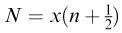if x is even, and if x is odd.

We can summarise the conclusions as follows. For equal rows of n disks when (2 n + 1) r < b < (2 n + 2) r,

For unequal rows of n + 1 and n disks when (2 n + 2) r < b < (2 n + 3) r,

In all cases,

We can think of N as a function of the two parameters l/r and b/r. A few sample values are given in Table 9.8. (Why do we start at b/r = 3 and l/r = 4?)

For comparison, the corresponding figures for the four-point contact (square) pattern are given in Table 9.9.

Interpret the mathematical solution

We see that there is no clear winner; either pattern can be the more efficient, depending on the values of the parameters. Note that, for parameter values in between the integer values tabulated, the value of N may remain the same but the wastage will alter.

For the case l = b = 1, r = 0.05, quoted above, the six-point contact method gives

and b / r = 20 (an even integer); so the case of unequal rows ( n = 9, n + 1 = 10) applies and

The four-point contact pattern obviously gives 100 disks and is therefore inferior in this case. Table 9.8

Table 9.9