Figure 5.10

the value of the starting value X 0 leads to a sequence, which after a number of time steps, diverges more and more from the previous sequences until the two sequences become totally dissimilar. This is illustrated in Figure 5.10.

5.7 Using spreadsheets

A computer spreadsheet is an ideal tool for investigating models based on difference equations because each cell can be made to reference other cells exactly as required. Formulas can then be copied to give as much as we want of the time development of the model, which can also be converted into graph form. Any parameters appearing in the equations can be assigned to separate cells and the effects of changing the parameter values immediately revealed. This has already been indicated in some examples in chapter 2.

Example 5.8

Suppose we decide to use a simple discrete first-order linear population model to predict the growth of a population which is presently 10 000 and we want to investigate the effect of birth rate and migration on the population growth. If we take annual time steps the modelling equation is

where b % is the net annual birth rate and m (individuals per year) is the migration rate.

In the spreadsheet we can put b and m in cells A1 and A2 and name them as b and m. Column B can be used for the population values (or if preferred, B for the n values and C for the P n values). We put the initial population value 10 000 in cell B1 and in B2 we type the formula = (1+0.01*b)*B1+m. We then copy this formula down the B column.

One of the advantages of spreadsheets is the dynamic linking between various components in the sheet. We can produce a graph to show how P n varies with n and any changes we make to the values of parameters such as b and m in the previous example produce instant changes in the chart. It is particularly instructive to do this for the chaotic examples in section 5.6 and observe the effects of altering the value of the parameter a on the resulting graph.

Example 5.9

Suppose that at the beginning of this year you invested £2000 in an account which pays interest at 9% p.a. At the end of the year, and subsequently every 12 months you withdraw £250.

1.When will you run out of money?

2.How does the answer to (a) change if you only withdraw £200 per year?

3.How much should you invest to pay your university tuition fees over the next three years if fees are £5000 p.a. payable at the beginning of each year?

The model we need is a difference equation satisfied by X n , the amount of money in the account at the end of n years (just after withdrawing money). This is X n +1 = 1.09 X n − w. We can put 250 for w in cell A1 and name it w. Putting X 0 = 2000 in cell B1 and typing the formula = 1.09*b1−w in B2, we then copy this formula down the B column. We find that we can reach the year n = 15 before our account becomes negative. To answer (b) we just have to change w to 200, and if we have gone down far enough in the B column we find the answer is 27 years. For part (c) w has to be 5000 and there is another difference in that we now want X n to represent the amount of money in the account at the beginning of the n th year. This time we want to find what X 1 should be so that X 3 = 0. Experimenting with various values for X 1 , we find the required figure to be £8795.56 so the initial sum that we need is £13 795.56.

Exercises

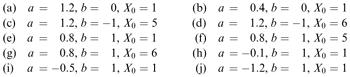
For the difference equation X n +1 = aX n + b (i) predict the results and (ii) confirm your predictions by using a spreadsheet to calculate the values X 1 , X 2 , … X 20 in each of the following cases:

5.1

Suppose that pollution has an adverse effect on the fish in Example 5.2, which can be modelled by

5.2a death rate directly proportional to the volume of pollution in the lake. Write down equations satisfied by F n and P n the size of the fish population and the volume of pollution after n years.

5.3Suppose that during every day of an epidemic:

1.x % of ill people die, and

2.y % of ill people recover and become immune, and

3.z % of susceptible people become ill.

Let

I n = number of ill people on day n

S n = number of susceptible people on day n, and

R n = number of recovered and immune people on day n.

Which three of the following options are consistent with assumptions (i)−(iii)?

1.I n +1 = I n − ( x /100) I n − ( y /100) I n + ( z /100) S n

2.I n +1 = I n + ( x /100) I n − ( y /100) I n − ( z /100) S n

3.S n +1 = S n − ( x /100) I n − ( y /100) I n + ( z /100) S n

4.R n +1 = R n − ( x /100) I n − ( y /100) I n + ( z /100) S n

5.S n +1 = S n − ( z /100) S n

6.R n +1 = R n + ( z /100) I n

7.R n +1 = R n + ( y /100) I n

8.S n +1 = S n + ( y /100) I n

Two adjacent islands A and B both have populations of gulls and there is constant migration of

5.4birds between the two islands. Suppose the net intrinsic growth rates are 5% on A and 3% on B. Let the total number

of birds on A in year n be A n with a similar notation for B. Suppose also that there is a constant migration of 1000 birds every year from A to B and 800 birds/year in the reverse direction.

Which two of the following options are compatible with the stated assumptions?

1.A n +1 = A n − 1000

2.A n +1 = (1.05) A n

3.B n +1 = B n − 800

4.B n +1 = (1.03) B n

5.A n +1 = (1.05) A n − 200

6.A n +1 = (1.05) A n − 1000

7.B n +1 = (1.03) B n + 200

8.B n +1 = (1.03) B n − 800

5.5Let X n = amount owed on a mortgage after n years,

m = monthly repayment,

N = number of years required to settle the debt, and

r = annual % interest rate charged on the amount outstanding.

1.Write down a difference equation satisfied by X n .

2.Use a spreadsheet to show that if the interest rate is 11% then the monthly repayment on a loan of £50 000 to be repaid over 25 years is £494.75.

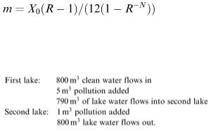
3.Show that if the mortgage is to be repaid completely in N years, the monthly repayment required to achieve this is

Suppose that the flow rates for the two lakes in Example 5.5 do not balance so that the lakes do not contain constant volumes of water. Let these volumes be A n and B n . Write down appropriate difference equations for A n , B n , P n and Q n given the following information about daily rates.

5.6

Glass X contains 20 spoonfuls of wine and glass Y contains 20 spoonfuls of pure water. One spoonful from X is added to Y and the mixture is stirred. A spoonful of the mixture is then transferred to X. Let X n = % of wine in glass X after n spoonfuls have been transferred in this way and let Y n = % of wine in Y. Find

5.71. a difference equation satisfied by X n

2.expressions for X n and Y n in terms of n

3.what happens eventually.