

are many situations like this where the use of mathematics provides valuable information concerning the behaviour of a system at much lower cost than an alternative ‘trial-and-error’ approach.
In road and traffic research laboratories, many traffic flow situations are analysed theoretically. Data are collected on the speed, size manoeuvrability of vehicles, traffic density and junction configuration. Relations between the essential variables are then drawn up using mathematical and statistical techniques. From examination and interpretation of the results the best roundabout configuration at some particular junction can be predicted. We say that the researchers have ‘built a model’ of the roundabout – not a physical model but a mathematical model. The model would usually be converted into a computer simulation, which could then be used to evaluate other similar roundabout designs. Other people within the laboratory will be capable of using the model, but it is the skill of constructing the model in the first place that we wish to capture.
Enough has been said now to give an idea of what mathematical modelling is and why it is so important. Exact definitions are not essential at this stage, but you will notice that it is easier and more useful to explain the process of modelling than to ponder on exactly what we mean by a model. Any model (including a physical model) can be defined as a simplified representation of certain aspects of a real system. A mathematical model is a model created using mathematical concepts such as functions and equations. When we create mathematical models, we move from the real world into the abstract world of mathematical concepts, which is where the model is built. We then manipulate and ‘solve’ the model using mathematical or statistical techniques. Finally we
re-enter the real world, taking with us the solution to the mathematical problem, which is then translated into a useful solution to the real problem. Note that the start and end are in the real world.
It is also important to realise at the outset that mathematical modelling is carried out in order to solve real problems. The idea is not to produce a model that mimics a real system just for the sake of it. Any model must have a definite purpose, which is clearly stated at the start. This statement may itself vary according to the point of view of the model user and there could in some cases be a clash between opposing groups regarding the particular objectives involved. For example, the effect of a new road bypass on a town centre traffic jam could be viewed differently depending on whether we side with the drivers, the pedestrians, the shopkeepers or the persons over whose land the new road will be built. It is possible that the model construction will be affected by such viewpoints, although generally it will not be the modeller's job to make a moral judgement on the issues.
It must not therefore be thought that for a particular problem there is one right and proper model. We are not in the same situation as with arithmetic or algebra, where, to each question, there is one correct answer. Many different models can be developed for tackling the same problem. (It is also true, and a remarkable demonstration of the power of mathematics, that the same abstract model can often be used for quite different physical situations.) Some models may be ‘better’ than others in the sense that they are more useful or more accurate, but this is not always the case. Generally the success of a model depends on how easily it can be used and how accurate are its predictions. Note also that any model will have a limited range of validity and should not be applied outside this range. This range could be a cost or resource or perhaps a mathematical restriction where a parameter must be non-negative.
1.3 The learning process for mathematical modelling
It is easy to describe real modelling problems undertaken by the professionals, but how are you to begin to develop your own expertise? As you start to work through this book, you are probably reasonably confident about elementary calculus, algebra and trigonometry and perhaps also some statistics and mechanics, but constructing mathematical models is a different matter. This book aims to help you to learn how it is done. It is not necessary to attempt complicated modelling problems based
on industrial applications. The ‘art and craft’ of model building can be learned by starting with quite common-place situations which contain a mathematical input based only on the mathematical work done at secondary-school level. As experience and knowledge are gained both in conventional mathematics and statistics as well as in
modelling, then increasingly demanding problems can be considered. The first examples need not be contrived or false, for there are plenty of simple real-life situations available for study. Within chapter 2, 12 such examples are investigated.
By the time that you have worked your way through to the end of this book, you should have gained considerable experience of mathematical models and modelling. It is important to do modelling yourself, to try out your own ideas and not to be afraid to risk making mistakes. Learning modelling is rather like learning to swim or to drive a car; it is no good merely reading a book on how to do it. Similarly, with modelling, it is not sufficient to read someone else's completed model. Also mathematics has perhaps acquired a reputation for being a very precise and exact subject where there is no room for debate: you are either right or wrong. Of course, it is entirely appropriate and necessary that mathematical principles are based on sound reasoning and development but, when we come to model some given problem, we must feel free to construct the model using whatever mathematical relationships and techniques seem appropriate, and we may well change our minds several times before we are satisfied with a particular model.
It is often important, for the best results, not to work on your own. In industry, it is normal for a team of people to work together on the same model, and the team may consist of engineers or economists as well as mathematicians. It should be the same for beginners at the student level; although you may read this book by yourself, we hope that most of the modelling exercises are tried amongst a group. Different people have different suggestions to make, and it is important to pool ideas.
To be a successful mathematical modeller it is not sufficient to have expertise in the techniques of mathematics, statistics and computing. Additional skills have to be acquired, together with the following general qualities: clear thinking, a logical approach, a good feel for data, and an ability to communicate and of course enthusiasm for the task!
Summary
1.1Mathematical modelling consists of applying your mathematical skills to obtain useful answers to real problems.
1.2Learning to apply mathematical skills is very different from learning mathematics itself.
1.3Models are used in a very wide range of applications, some of which do not appear initially to be mathematical in nature.
1.4Models often allow quick and cheap evaluation of alternatives, leading to optimal solutions which are not otherwise obvious.
1.5There are no precise rules in mathematical modelling and no ‘correct’ answers.
1.6Modelling can be learnt only by doing.
CHAPTER 2
Getting Started
Aims and objectives
A selection of modelling problems is presented in this chapter. There are 12 in all, taken from a wide range of application areas, and with a variety of demands on the user. Some mathematical background and technique is required for these 12 problems, such as that normally found in the first year of a mathematics degree course. This means an awareness of basic calculus, geometry and trigonometry. Also some knowledge of elementary matrix algebra, probability and statistics will be assumed. Simple kinematic relations are also drawn upon as necessary.
The overall objective is to get an idea of what mathematical modelling is about.
2.1 Introduction
Mathematical modelling is an active pursuit that can only be learned by doing it yourself (or in a small group). Getting started may be the big step – a bit like swimming – once launched safely and backed by some success then confidence grows and also mathematical robustness and maturity. Whilst the overall point in teaching mathematical modelling is to help train applied mathematicians (for industry and business), we can make a start at undergraduate level. There is no need to wait to try modelling until you have three or four years of university training behind you. There is every reason to start early in the degree programme and gradually build up experience and the necessary skills.
The 12 examples are intended to show what mathematical modelling is about in practice. The problems are not all equally difficult or of equal length to ‘solve’. We must be careful about using a term like ‘solve’ since in modelling there is often no single answer to the problem in the conventional manner. Alternative approaches can often be found to those given in the examples and this is quite normal in mathematical modelling. Sometimes there are ‘second thoughts’ about a particular problem, first setting up a simple model but then modifying it by introducing more sophisticated techniques depending on the level of mathematics you possess. This progression will be considered again in the next chapter. Thus in the spirit of ‘Getting Started’ all the examples below are all presented in a straightforward manner.
2.2 Examples
Example 2.1 Data fitting
(a) Bird life longevity Problem description
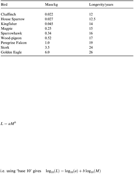
Ornithologists have an important role in nature conservation and in the protection of bird life generally. Collecting and understanding data on bird life helps in this protection work. One useful investigation concerns the normal life span of common British birds and whether there is a general model that can be formed to relate ‘longevity’ with ‘body mass’. Data is available as shown in Table 2.1.
Table 2.1
Model formulation
This is a simple data-fitting situation in which we are interested in finding out whether a model formula can be evaluated to relate longevity with body mass. Denoting the bird longevity by L (years) and the body mass by M (kg), the idea is to construct the model in the simplest way that is reasonable. In order to appraise the situation first, a scatter graph of the data is necessary. This can easily be produced using a spreadsheet package (such as Microsoft Excel) or drawing by hand. A spreadsheet package is an important modelling tool that will be referred to many times in this text. Here the subsequent attempt to obtain the bird formula can be simply carried out using spreadsheet facilities.
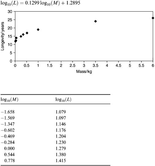
Figure 2.1 shows the outcome from the scatter plot, taking mass as the input variable ( x -axis) and longevity as the output variable ( y -axis)
The results indicate a concave downward effect for the possible relation we are seeking. It is reasonable to assume the obvious fact that ‘ M = 0 implies L = 0’ and so we shall look for the model in the form:
(2.1)
where a and b are constants to be determined. This choice of an algebraic formula seems reasonable; we expect b to be < 1.0 (and positive). Since there is no inherent ‘growth’ or ‘decay’ feature present in the original problem it is reasonable not to use exponentials in the construction. Having obtained the relation (equation 2.1), it could be used to predict longevity of other bird species.
The next step is to attempt to calculate values for a and b and this is done by taking logarithms. This well-known procedure is very important in analysing data and obtaining resulting model fits. We can use either ‘base e’ logs or ‘base 10’ without loss; in either case the original suggested formula is linearised:
(2.2)
Hence if the bird data does agree with equation (2.1) then equation (2.2) will be a straight-line graph when log 10 ( M ) is plotted against log 10 ( L ).
Taking logarithms to base 10 produces Table 2.2. On carrying out the plot we obtain the outcome shown in Figure 2.2.
The graph shows the fitted straight line and gives the equation of the line in local ( x, y ) coordinates together with a measure of the quality of the fit obtained. We may have to draw in the ‘line of best fit’ by hand, but a spreadsheet package will automatically calculate this using the ‘least squares principle’.
In this case the outcome is that:
(2.3)
Figure 2.1
Table 2.2
while the R 2 value close to 1.0 indicates a good fit.
Should this linear fit be poor – indicated by a low R 2 and also visually in Figure 2.2 by a clear noncolinearity in the data – then this would suggest that the original proposed model (equation 2.1) is invalid. We must abandon the attempt to relate longevity with mass using equation (2.1) or try an alternative model formula. This data-fitting activity can be examined further in many standard texts in statistics as ‘regression analysis’. See, for example, the text by W. W. Daniel and J. C. Terrell listed in the Bibliography.
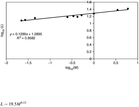
Figure 2.2
The objective was to calculate values for the original constants a and b for the model.
From equations (2.2) and (2.3) it can be seen that b = 0.1299  0.13 and log 10 ( a ) = 1.2895, giving a = 19.47
  19.5. Thus finally the bird model formula is:
(2.4)
Interpretation
1.How good is this finished model and what would be its use? It can be seen as a rough guide only despite the evident goodness of fit shown in Figure 2.2. Only nine data pairs are available therefore adding more data would give greater confidence to the outcome. The outcome shows something of the use of spreadsheet modelling.
2.Data measurement and accuracy (reliability) also play some part in this model. Note that the mass data is quoted to two significant figures and longevity to the nearest half year. Is this reasonable? The figures stated here will have been averaged from ornithologists’ collected data. We note that the mass of the eagle is about 270 times that of the chaffinch!
The final result should not contain a precision greater than the input data. A further concern for the ornithological modeller is that bird mass will vary depending on bird habitat. On the other hand by including both the eagle and the chaffinch we have some claim to getting an overall formula with some credibility.
(b)Athletics times
Problem description
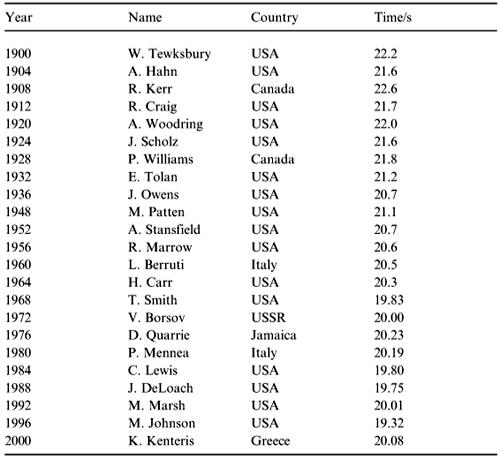
Sporting achievement is always interesting to measure as performances continue to improve and records are broken. In athletics track events winning times are coming down for both men's and women's races. In the Olympic Games the times achieved for the 200 m by both men and women make a useful investigation. Two questions of interest are (i) is there some limiting time below which it will be impossible for any human to complete a 200 m race? and (ii) will the winning times of women always be inferior to men? Data is available from 1900 for the men's 200 m Olympic Games winning times and from 1948 for women.
Model formulation
The data is readily available and is given in Tables 2.3 and 2.4. We have to examine and analyse the data by first graphing it following a similar procedure to that previously described.
From Table 2.3 we can notice the preponderance of USA winners in this event and also that the times have been descreasing although not continually (or monotonically). This data is of a different nature to that used in the previous example in that it is a time series. Also modern measuring techniques mean that the times given are reliable to the quoted precision. Note that since 1968 it has been possible to measure correct to the nearest onehundredth of a second. It is practically impossible to imagine what 0.01 s actually records, but to help we can calculate how far a runner will travel in 0.01 s:
Table 2.3 Men's 200 m Gold medallists
Table 2.4 Women's 200 m Gold medallists
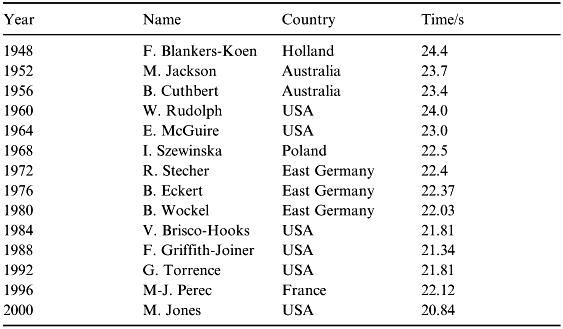
Running 200 m in (say) 20 s gives an average speed of 10 ms −1 so the athelete travels 10 × 0.01 m in one-hundredth of a second = 0.1 m = 10 cm. This is a realistic viewable gap between athletes provided the finish can be photographed. It would seem that a time quoted correct to three decimal places (in seconds) is not realistic.
In order to answer the two questions (i) and (ii) posed in the problem description, we will try to model the patterns of the data. Again a ‘scatter’ graph plot is the place to start (see Figure 2.3).
A downward trend is shown for both men and women as expected. We notice that the performance in both the men's and women's event has slightly deteriorated since 1988. Nevertheless there is visual evidence that the two data sets are closing up.
To return to the modelling task and the two questions posed; there is a prediction feature to answer. One of the important uses of mathematical modelling is essentially about making reliable and useful predictions. This occurs in supply and demand examples (water and power), rocket and payload behaviour (before launch!) and money market tactics to name some obvious situations. It can be very expensive to ignore the effectiveness of a good mathematical model to help in decision making if a mistake is subsequently made through merely backing a hunch, which proves to be wrong.
Thus the issue here is to predict from the given data what winning times will be achieved in the future. Looking at the graph in Figure 2.3, we wish to extrapolate forward over the next 20 or 30 years or so and obtain answers to (i) and (ii).
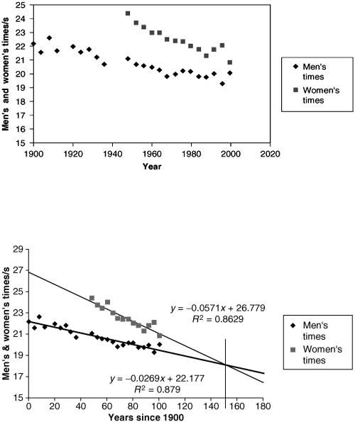
Figure 2.3
Following on from Example (a) we shall fit a model formula to each data set using spreadsheet tools. By looking at the data a simple linear fit for the original raw data can be carried out since neither set suggests clearly any alternative fitting function (see Figure 2.4).
Figure 2.4 Interpretation
The outcome shown in Figure 2.4 epitomises some of the dangers of predictive modelling. Linear models for the 200 m times may be acceptable over the periods covered by the data, but what credibility can be placed on times predicted in years ahead? The steady fall in winning times for the men's race
indicates that ultimately y = 0 at x = 22.177/0.0269 = 824. Thus using the model, the race is run in zero time in the year 2724 AD. This indicates no limiting time for runners at all which seems unreasonable! Thus question (i) has not been satisfactorily answered so far using the suggested models. With regard to (ii), we can say something. Looking at Figure 2.4 it is clear that the fitted line for the women's race is steeper than that for the men. The more rapid improvement shown in women's performance could indicate a closing up in winning times with the men so that there would be equality by about the year 2050 if performance improvement continued at the same rate.
Returning to question (i), we must conclude that the linear model is only valid for a limited range of
years. Obviously a different model would seem more suitable such as
where T is the time achieved (s), t is the number of years since 1900 and a, b and c are the model parameters to be calculated. Fitting the second of these models would provide for a limiting time value, c, which is more plausible than the other alternatives. Either c has to be estimated first and then the procedure in Example (a) used, or a more complicated numerical method invoked to fit the model directly to the given data.
We shall retrun to issues of fitting a model to data in chapter 8. Example 2.2
Windscreen wipers Problem description
Having considered modelling involving data collection and interpretation in Example 2.1, we turn now to a simple spatial investigation. The effectiveness of car windscreen wipers is a suitable topic for examination since there is a measuring element involved and there is a plentiful number of available vehicles all with different wiper configurations at the front and back. Generally cars have two wipers overlapping on the front screen and one wiper at the back. Also most wiper arms are bent, presumably to make the pivot position more convenient for car body designers. In a modelling investigation there is a need to identify the actual problem that we are trying to solve. There are a number of interesting problems relating to windscreen wiper action, but here we shall concentrate on a single bent wiper, say positioned on the rear window. The particular problem will be to investigate the advantage in fixing a bent wiper when the pivot is not centrally placed.
Model formulation
A diagram of the situation is needed and is shown in Figure 2.5.
The investigation requires an expression for the area of window wiped by the blade. This will depend on the size of wiper blade, angle of rotation and so on. It is useful to make a list of all those quantities that will be needed to obtain the area expression. It will become clear as mathematical modelling techniques are developed within this textbook that drawing up a comprehensive list of factors and variables for a given modelling task is essential to good modelling practice. Further the variable list allows us to choose symbols for each item and also to indicate an appropriate unit for that item. For the windscreen wiper problem some required variables can be marked on Figure 2.5 but it is still necessary to draw up the formal list (see Table 2.5).
There is another issue creeping in here which epitomises the skills of the mathematical modeller. We are obliged to make assumptions to simplify the problem before we can proceed much further. The initial situation has to be refined so that it can be formulated into effective mathematical relations and formulae, i.e. a model is created. It may be thought that there is some ‘cop-out’ from the original problem by introducing simplifying assumptions, but as we shall see later in the book it is almost always necessary to refine the original real-world situation as the first modelling step before conversion into mathematics. It is a bit like ‘learning to walk before learning to run’ but we shall return to this point in the next chapter. Introducing simplifying assumptions does not mean that an enfeebled model is produced. The outcome from the first
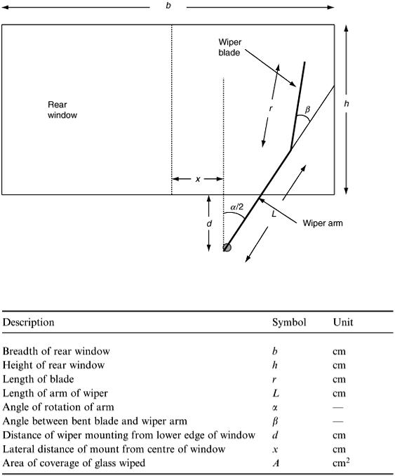
Figure 2.5
Table 2.5 Windscreen wiper variable list
model will probably cause us to review the assumptions before trying again and creating a more complex model.
Now what assumptions should be made so that a suitable first model can be formulated? On examining a range of vehicles, the position of the rear window blade varies from car to car. Also the size and shape of the windows vary considerably.
The particular assumptions we make will often be the subject of disagreement between modellers and so some care must be taken in selection. The following assumptions will be introduced for this investigation:
1.The wiper mount will be taken at the base of the window; hence referring to the variable list, d = 0.
2.The shape of the window will be taken as rectangular (as drawn in Figure 2.5).
3.The wiper arm executes symmetric sweeps of ±α/2 degrees either side of the vertical.
The first of these assumptions seems quite drastic particularly as this is not the situation for most vehicles. Also assumption (iii) may be incorrect since the actual sweep is not symmetric. However, as has been noted already it is good modelling practice to simplify the situation even if a highly significant feature is omitted, albeit temporarily. This can separate key features in the problem to the benefit of the trainee modeller and these can later be recombined into a more sophisticated model.
As the wiper blade performs its cycle, circular areas are mapped out. We require the area shaded in Figure 2.6 and so we should set out to calculate this.
From circle mensuration formulae, the area of a sector of a circle of radius a and subtended angle θ is given by  a 2 θ. (Consult the mathematical dictionary listed in the Bibliography.)
Now referring to Figure 2.6, there is an area APR which will not be wiped, since the wiper arm is bent through the angle β and also assuming (iii) above. However, this area is repeated at the other end of the wiper sweep where it is added in again, so the area to be calculated is, in fact, ARR′A′.
This area, using the sector formula = 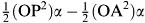
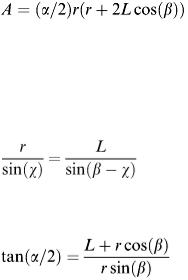
The length OP has to be evaluated from the triangle OAP and using the cosine rule we have OP 2 = L 2 + r 2 + 2 Lr cos(β).
With OA = L and simplifying the expression we have finally:
(2.5)
The use of this formula depends on what restrictions are imposed from the dimensions of the window and also the position of the wiper mount and angle of bend of the blade. Some restrictions are now investigated below.
For instance, the wiper blade at the left end if its sweep cannot overstep the glass area. A condition can be obtained so that this is achieved. From Figure 2.7, using the sine rule in the triangle OA′P′:
Rearranging and using  gives the relation:
(2.6)
This latter equation indicates a limitation on α in terms of β if L and r are considered fixed. Further limitations on the wiper action can be examined from the requirement that the rotary action must remain on the window glass. Referring to Figure 2.5, two edge conditions may be evaluated, the first to prevent wiping outside the right-hand edge of the window and the second to prevent wiping over the top edge. These are easily seen from simple trigonometry to be respectively:
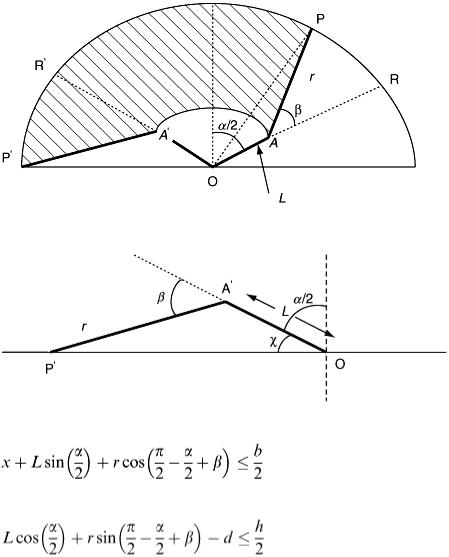
Figure 2.6
Figure 2.7
and
(2.7)
Interpretation
There is scope here for examining the real situation by taking measurements for particular vehicles. Data can be collected from a wide variety of cars and compared for wiper effectiveness. By effectiveness we shall evaluate the area of rear window actually wiped as a percentage of the total window size. Two well-known Vauxhall models will then be compared to see which is the more effective. It is noted in passing that conventional saloon cars usually do not have rear window wipers. Note also from the assumption (iii), see Figure 2.6, the wiper arm rotation is indicated as sweeping to and fro symmetrically over the range (−α/2, α/2). This may not be the case for some cars where the sweep is inclined to the vertical. However, equation (2.5) will still hold since circular regions are always swept out. There will always be some restriction indicated by equations (2.6) and (2.7) to take into account. We can see there is a bigger modelling problem here concerning optimum wiper design for a given window; this would, however, widen the investigation to include cost features and a more detailed examination of what the wiper is meant to achieve.
The two vehicles considered here are the Vauxhall Vectra and the Agila. Data for the required variables is as shown in Table 2.6.
Calculation of the required percentages gives, using equation (2.5):
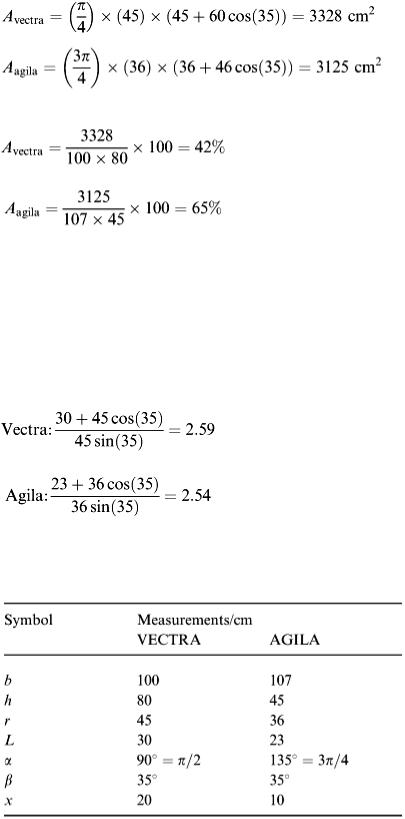
The area wiped by the Vectra wiper is slightly larger, but when the percentages are calculated we have:
Thus it proves that the Vauxhall Agila is the more effective in this simple test.
There will be some reservations perhaps in awarding the Agila wiper as superior to that of the Vectra. For instance we see that the Agila has quite a small rear window and considerably less overall rear vision. This brings the argument back to what the purpose of the rear window wipe is for. If it is the vehicle then it may be concluded that there is little difference between the two cars’ wiper performance since the ‘A’ calculations are almost equal. We notice that for both cases here the ‘x’ value is significantly positive. Finally the condition given by equation (2.6) can be tested.
The values of the right-hand side of equation (2.6) are respectively:
This indicates that the maximum value of α/2 is about 68° and this is satisfied for both models being considered. The two further edge conditions given by equation (2.7) are easily shown to be satisfied.
Table 2.6
An interesting extension of the windscreen wiper investigation is the case of two wipers (on the front windscreen) and the evaluation of how much of the windscreen is wiped twice during each cycle. The answer is provided in the ‘Solutions to Exercises’ section at the end of the book.
Example 2.3 Traffic lights Problem description
Keeping to the transport theme, we turn now to the motion of a stream of vehicles.
How many cars can pass through a set of traffic lights when they turn green for a period of 15 s? Suppose that a line of cars are queueing to pass through a junction and the lights are set at red. Often the queue is so long that a driver some distance from the front of the queue sees the lights go green and back to red again before even moving forward himself, let alone actually getting across the junction. The way in which traffic behaves at lights can be quite complicated, depending on such things as ‘right-turn filters’, ‘no left turn’ and so on. Also, when the traffic density decreases, often no queueing takes place at all, and the number of vehicles passing across a junction will depend on how many there are in the vicinity of the traffic lights in the first place. Here we investigate the saturation case where there is already a long queue of cars poised at a red light waiting to move off.
A number of assumptions will be made at the outset.
1.The junction is not blocked in any way.
2.All cars intend to pass directly across the junction.
3.All vehicles are cars of the same size, 5 m in length, and initially at rest.
4.There is a 2 m gap between each stationary car.
The objective is to calculate how many cars pass across the junction during one green light cycle. Model formulation
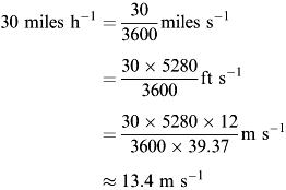
How does a car pull away? We assume that it will accelerate uniformly up to a maximum speed of 30 miles h −1 (the town speed understood by most drivers if not actually observed!) We have a mixture of units here; miles per hour must be converted to metres per second:
Reasonably, the final speed will be taken as 15 m s −1 . Next, the acceleration of a car in city conditions has to be assessed. Some car manuals claim ‘0 to 60 miles h −1 in 10 s’. Using this, we get 60 miles h −1 = 26.8 m s −1 achieved in 10 s; so the acceleration is 26.8/10 m s −2 = 2.68 m s −2 . Acting a little conservatively, we shall take the acceleration to be 2.0 m s −2 .
On the assumption that, once the final speed has been reached, this speed is then held constant, we can draw a velocity–time graph (Figure 2.8).
Hence after 7.5 s the car has reached its final speed of 15 m s −1 . Now describing the motion of one car is not sufficient for the objective of the model – the motion of the rest of the queue must be considered as well. Suppose there is a delay of 1 s in thinking time before the next car reacts and pulls

away. This motion is easily incorporated into the same velocity–time graph, and all following cars can be similarly marked in (Figure 2.9).
The distance travelled by a car can also be conveniently evaluated from a velocity–time graph by calculating the area under the graph. Thus, after 4 s, we have
Figure 2.8
However, where are these cars in relation to road markings at the traffic lights? Measuring from the front bumper of each car, we can draw up a table of car positions, both initially and after 4 s (Table 2.7).
Now after 7.5 s the situation changes since some cars will have reached their maximum speed of 15 m s −1 . Can you work out a general formula for the distance s metres that each car has travelled after, say, T seconds?
A suggested formula is
(2.8)
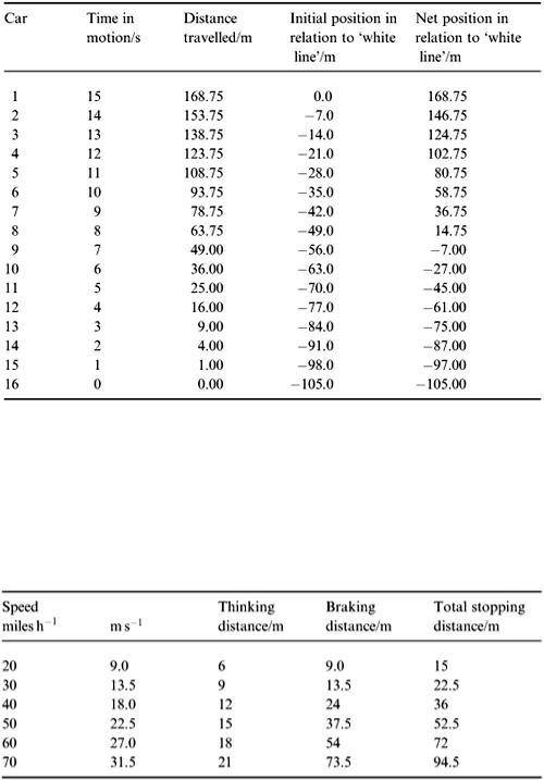
Next suppose that the lights stay green for 15 s; can you calculate how many cars pass through the junction? The situation at T = 15 is shown in Table 2.8.
You can use the table to calculate how many cars pass through before the lights are set at red again.
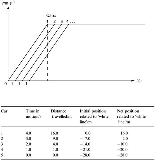
Figure 2.9
Table 2.7
Interpretation
From the last column in Table 2.8, we can see that eight cars certainly pass through the traffic lights.
The ninth will probably also go across since it is travelling at 14 m s −1 (  31 miles h −1 ) at the time limit of T = 15 s and it is only 7.0 m behind the ‘white line’. We can see here the reason for an amber light so that this marginality can be allowed without mishap as this car goes through.
[Note that from equation (2.8) the maximum allowed car speed is 15 m s −1 (33.5 miles h −1 ) which due to our earlier assumptions is greater than the maximum town speed permitted.]
The tenth car has sufficient distance (27 m) to spare before the ‘white line’ and should stop. Stopping distances can in fact be calculated in terms of car speed by modelling retardation rates. The data is usually printed in the Highway Code booklet and is given here in Table 2.9.
From Table 2.9 we can see that stopping distance for a speed of 31 miles h −1 is about 23 m.
There is great potential for simple mathematical model building when considering streams of cars. For example:
Table 2.8
1.Considering a line of moving traffic entering, say, a long tunnel, what is the speed that the cars should travel so that the maximum number of cars pass through the tunnel per hour?
2.Given that there is a stretch of road under repair preventing the normal two-way passage of cars, and so necessitating the setting up of temporary traffic lights, what light sequence must be used so that the most cars will pass by the repair section per hour?
3.When is it safe to overtake?
Table 2.9 Stopping distances
Example 2.4 Price wars
A common occurrence in retailing is competition between rival establishments over which shop can claim most of the market. Market share can be affected by advertising locally, by price variation and by sales gimmicks, etc. The most straightforward price war situations occur in supermarkets or in garages. Here a petrol sales price war is considered.
Problem description
Two petrol stations operate from adjacent main road sites and vie with one another for business. Competition is also stiff from other petrol stations not far away and profit margins from the sale of petrol are very sensitive to sudden changes in demand. On the other hand, the market is large and, although both petrol stations have regular customers, they realise that many of their sales are to ‘casual’ drivers.
One day, one of the petrol stations suddenly drops the ‘price per litre’ as advertised on the station forecourt in an attempt to attract more of the market. The other petrol station immediately notices a fall in trade as a result. They decide that they must follow suit in dropping the price and so start up a ‘ price
war ’ with the first garage. The second garage wants to devise a strategy so that, in altering their price, earnings will be as high as possible.
Model formulation
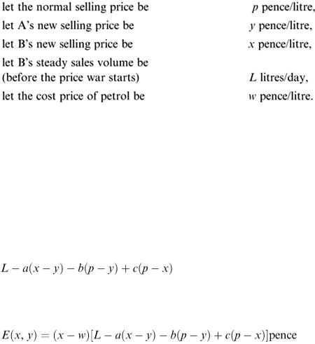
Let the first garage be denoted by A, and the second by B. The crucial part of setting up a model here is to attempt to predict how B's market share will be affected by the sudden price drop by A. We have also to take account of the ‘normal price’ of petrol still being charged by other garages. To quantify these ideas, we introduce some notation:
Now this example is typical of a more ‘open’ situation where we have to speculate on the behaviour and relation between variables. This is one of the skills that we are going to need if we are to become effective mathematical modellers.
To build a model of sales volume variation, we now assume that B's daily sales are affected as follows. Sales are changed by an amount directly proportional to the following.
1.The difference between B's price and A's price.
2.The difference between B's price and the normal price.
3.The difference between A's price and the normal price. Thus our model for the new daily sales for B is
where a, b and c are proportionality constants. Note that a, b and c must all be positive. An ‘earnings function’ can now be calculated for garage B, since earnings are given by ‘price × sales volume minus costs’. Hence the daily earnings of B are
This expression can be maximised as a function of x, regarding y as an input parameter. It is easily shown by elementary calculus that the x value for maximum E is
The model is now tried with data as follows:
(Prices can vary owing to tax and market features.)
The proportionality constants are our main worry and have to be estimated in some way or other. (This often happens in mathematical modelling.) This particular model would need real data to enable a, b and c to be fixed, but at this stage we are concerned with principles as much as accurate data collection. It is quite instructive to judge what size of parameter to select for a, b and c. By examining the relative sizes of the quantities within the sales function, we decide to choose a = 4000, b = 500 and c = 1000. You should be able to see that taking a = 1.0, or 0.2, say, will not be sensible. Also we might expect that the terms containing a, b and c are not equally important, i.e. it is not necessary to choose the proportionality constants all equal.
Interpretation
Using the above values provides sensible results, which are ideally presented on a simple spreadsheet, as shown in Table 2.10.
These results give the daily price (in the second column) that garage ‘B’ must sell at in order to maximise its earnings. We can see that for this model, its daily earnings will drop below that previously achieved before the price war when ‘A’
Table 2.10 Price war
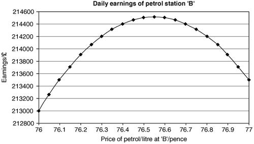
Figure 2.10
decides to sell at 78 pence (or less). The earnings function is a quadratic in x for a given choice of y. Its behaviour is shown in Figure 2.10 for the case y = 79.
There is a ‘family’ of quadratics for varying values of the parameter ‘ y ’. Notice that B's new maximum daily earnings are soon in debit compared with their old earnings as A's price drops. The choice of the parameters a, b and c will obviously affect the outcome, and it can be argued that the values chosen for the parameters are no longer correct beyond a certain price cut.
Example 2.5
Evacuation
From time to time, any organisation occupying a large building will want to practise an evacuation procedure in case of an emergency. The evacuation may be required for a variety of reasons but in all cases will have to be organised to proceed in an orderly manner.
The people whose responsibility it is to check the safety of the arrangements for evacuation will want to make sure that in each room there are clear instructions on how to leave the building. They will also want to have some idea of how long it will take for the building to empty. This will then enable them to decide whether the number of exit routes are sufficient to cope when the building is full to capacity.
To avoid having too many practice evacuations, it is helpful if an estimate for the total exit time can be made by trying a theoretical approach instead. This is where a useful modelling exercise can be developed.
Problem description
The above general issues are rather difficult to deal with since we shall need to know how large the building is, how many exit stairs are available, how many people per room and so on. However, a good modelling tactic is to consider a simplified problem when the original seems too hard or too undefined. Often the outcome from a simpler situation is contributory to the main problem anyway.
Consequently, we shall take the building to be a school or college and confine attention to one floor where there are a number of similar classrooms in a row. Suppose that each is evacuated by walking along the corridor serving the rooms and then through the exit door at the end. The situation is shown in Figure 2.11.
The objective of the simplified problem is to work out how long it takes for the four rooms shown to be completely emptied and the occupants all to pass through the exit door.
Model formulation
It is instructive first to consider an orderly departure from a single room. A list of the relevant variables helps to clarify the situation:
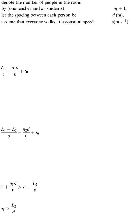
Thus there is a chain of people of length n 1 d m filing out of the room. On the assumption that the leader of the chain starts at the door, then the time needed for everyone to leave is n 1 d/v.
There will be an initial short delay while the first person reaches the classroom door. Denoting this by t 0 , then we have the total room emptying time of n 1 d/v + t 0 . At this point, the last person has just reached A in Figure 2.11; so, as there is still a distance L 1 to walk to the exit door, an additional time of L 1 / v is needed for this. Thus, finally the total time for the first room to evacuate is
(2.9)
This is all quite straightforward, but we have only considered one room. Now refer to the second room, which could be a different size from the first and contain a different number of people. It is likely that t 0 will be the same, and v
and d also the same. Given that there are n 2 + 1 people, then the chain of people for the second room takes n 2 d/v + t 0 for the last person to reach the door of the classroom.
The corridor length that this second chain has to walk along is L 1 + L 2 m, from point B to the exit. At a speed of v m s −1 the time needed for this is ( L 1 + L 2 v ). The total evacuation time from the second room is
(2.10)
However, there is a fallacy in this analysis, since no account has been taken of the possibility that the two chains will conflict in the corridor. Normally, corridors are sufficiently wide for at least two columns of people to walk side by side. We shall suppose for safety, however, that in this situation there is only enough width for one column to occupy the corridor at a time. This means that a delay can occur at point A when the second chain is held up while the first is still leaving.
The time for the leader of the second chain to reach point A is t 0 + L 2 / v and the time for the last person in the first chain to reach point A is t 0 + n 1 d/v. Hence a delay occurs when
i.e.
(2.11)
On the assumption that there is a delay, then the second chain joins on the end of the first. The total time now is
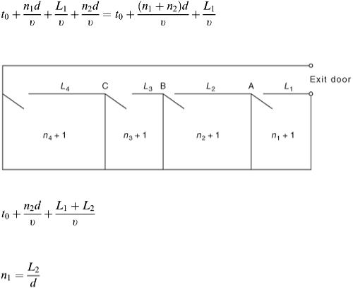
(2.12)
If no delay takes place, then n 1 is too small (for example) and the total time for evacuation is the result from equation (2.10), i.e
Figure 2.11
(2.13)
Finally, we can calculate the evacuation time when the chains blend together without a delay or a gap, i.e. when
(2.14)
In this case, equations (2.12) and (2.13) are identical. Interpretation and further development
Data is taken as follows. Let L 1 = 10 m, L 2 = 12 m, v = 2 m s −1 , t 0 = 3 s and the space gap d = 1 m. Suppose that the number of people in the first room is 13 and that the second room contains 31 persons so that n 1 = 12 and n 2 = 30. The evacuation time can now be calculated from equation (2.13) as 3 + 30 × 1/2 + (10 + 12)/2 s = 29 s, condition (2.14) holding in this case.
Only two of the rooms have been considered in this calculation. Assumptions have been introduced about the corridor width here and so on.
The simple calculation is, however, a start. More realistically we are interested in the evaluation of a multistorey building (or perhaps an aircraft). Whilst the actual procedure may contain alternative tactics motivated by a degree of panic, the ordered evacuation model begun here gives a useful guide to the situation. It gives (probably) the minimum evacuation time for a given circumstance.
However, armed with a suitable simulation tool, it is possible to analyse more complicated evacuation problems. A taste of what is possible is shown below where say, students evacuating from two adjacent lecture rooms merge in an orderly fashion at a foyer at the head of stairs before advancing downstairs to the next level.
The output shown has come from the package ‘MODELMAKER’ (Cherwell Scientific Publishing, Oxford at www.cherwell.com ), which is capable of solving dynamic models in terms of sets of differential equations. It may seem unrealistic to express our formalised evacuation process as differential equations, but it can be accomplished with good effect as described briefly here. The advantage of a computer model is clear, since it is relatively easy to extend the model to analyse evacuation of a large university building.
The situation is indicated by the MODELMAKER block diagram as shown in Figure 2.12.

Suppose there are 120 students in lecture room 1 and 180 in room 2. The students leave the rooms in an ordered manner at a fast walking rate as previously of 2.0 m s −1 (flow rates F1 and F2 on the diagram). Suppose further that the foyer capacity is at most 100 students, that the walking speed down the stairs is 1.0 m s −1
(flow rate F3) and that it takes 30 s delay for the first student to reach the bottom of the stairs. Suppose further that from lecture room 2 there is an alternative stairway to reach downstairs (flow rate F4) and that the delay in reaching the bottom is 40 s. Assume that both lecture rooms immediately begin to empty. We want to calculate how long it takes for everyone to get downstairs. MODELMAKER will evaluate this and display the output graphically as shown in Figure 2.13.
From Figure 2.13, it can be seen that DOWNSTAIRS2 fills after 125 s and contains 86 students, whilst DOWNSTAIRS1 takes until about 244 s to fill and contains the remaining 214 students.
Figure 2.12
Figure 2.13
With this evacuation scene it therefore takes 244 s before all 300 students are evacuated.
The MODELMAKER program for the evacuation problem is given in Appendix 1 at the end of this chapter.
Example 2.6 Corridors and corners Problem description
A familiar scene in hospitals with a surgical unit is the moving of a patient from the ward to the operating theatre whilst the patient remains in bed. In other words the bed is pushed along the corridor by hospital staff at a fair speed without inconveniencing the patient. Unfortunately, some hospitals have narrow corridors with right-angle bends in them. Suppose that there is just such a bend between the operating theatre and the wards. Beds have to be wheeled along this corridor, negotiating the rightangle bend.
Often for maintenance and decorating purposes, ladders and long planks also have to be carried round the hospital corridors. Again there is a right-angle bend to negotiate.
There is a modelling problem in both these situations. It is interesting to see what length of ladder can be carried round the corner and also whether a typical hospital bed can be comfortably pushed round. In the interests of saving space, and for future corridor design, we might want to find out what the minimum width of a corridor is so that a bed can pass round a corner.
Model formulation
A diagram (Figure 2.14) is helpful in this situation.
It seems reasonable that the problem of moving a ladder round the corner is best considered first. Having dealt with a ladder, the bed can then be investigated. Another diagram (Figure 2.15) is useful so that the ladder problem can be considered.
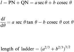
The problem is generalised so that, for corridor dimensions a and b and ladder of length l, what is the greatest value of l so that the ladder will still pass round the corner? (In practice the units of length will be taken in metres.) After some thought, we realise that what is required is the minimum value of PQ. From the trigonometry, PN = SN cosec θ and QN = RN sec θ. Hence, by addition,
(2.15)
Using differential calculus,
On setting d l /dθ = 0, the condition for a minimum is tan 3 θ = b/a. This means that the ladder length we want can be calculated by substituting the θ value into equation (2.14). This gives
(2.16)
(Note that, to get the longest ladder for given a and b, it is the minimum value of l that is wanted.) Substituting values for a and b into equation (2.16) enables the ladder length to be calculated. Now let us return to the bed problem (Figure 2.16).
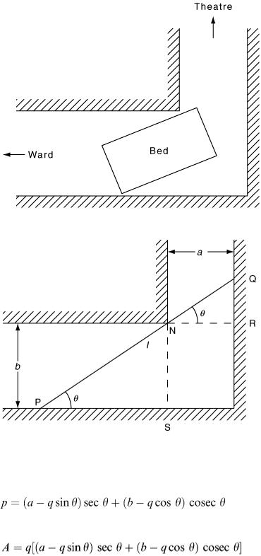
Figure 2.14
Figure 2.15
First, the area A of the bed is given by A = p × q. From the trigonometry in Figure 2.16 a relation connecting p and q can be obtained using AB = AN + NB:
(2.17)
Hence,
(2.18)
Although the objective here is to calculate minimum dimensions of a and b so that a standard bed can be pushed round the corner, it is more convenient as far as the mathematical model is concerned to tackle the problem the other way round and to treat p and q as variables for given a and b. In fact, p has been eliminated in equation (2.18); so we proceed with equation (2.18) regarding q and θ as variables. The approach is then analogous to that for the ladder, but the mathematics is a little harder. We attempt
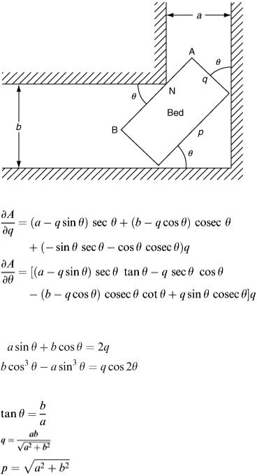
to minimise A in equation (2.18) using calculus but note that there are two independent variables to be differentiated, q and θ. Note that if q = 0, equation (2.17) becomes p = a sec θ + b cosec θ (compare with (2.15)), and equation (2.18) becomes A = 0 as required.
It is easily shown in calculus textbooks on functions of several variables that the minimum is sought by differentiating with respect to each variable in turn, while keeping the other constant. This technique is known as ‘partial differentiation’ and will probably be covered in a parallel first-year course. To indicate a partial derivative, a slightly different notation ∂ for the derivative is normally used.
Consequently, evaluating ∂ A /∂ q and ∂ A /∂θ gives
Figure 2.16
The required conditions for a minimum value of A are found by equating both these derivatives to zero. After a little manipulation the conditions reduce to
Solving for q and θ gives
(2.19)
(2.20)
(2.21)
Strictly from the calculus, we should now check that the conditions obtained do give the minimum A value and not the maximum. However, from reference to Figure 2.16, it can be seen that A can increase
without limit for small θ values; so we assume the solution in equations (2.19) and (2.20) corresponds to the required minimum.
Interpretation
The ladder result is easily evaluated for given values of a and b. We note at this stage that this example is a straightforward task in geometry and trigonometry where one specific correct answer is the outcome. Mathematical modelling is rarely like this! Normally we have to wrestle with assumptions concerning a particular situation, which have to be made before we can proceed. The assumptions will simplify the initial problem and will affect the usefulness of the outcome in reality. This has already been demonstrated in Examples 2.2–2.5.
Nevertheless there is some attraction in tackling Corridors and corners in this chapter since the effort in solving the situation will help to develop skills in employing a clear thinking approach, good diagrams and correct interpretation and validity of the results.
Confining attention to the bed problem and introducing test data, suppose that a standard bed has length 2 m and width 1 m. This means that p = 2 and q = 1 can be substituted into equations (2.20) and (2.21).
Simple calculation gives that 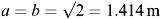
As has been noted this is really the inverse problem since the dimensions of the corridor will be known first! Thus suppose that we have a narrow corridor where a = 1.0 but b = 1.5. Again from equations (2.20) and (2.21) this gives p = 1.8 m and q = 0.8 m as bed dimensions. This bed is only 70.87 inches long and so will not suit a 6 ft patient!
Extensions are interesting with this example:
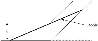
1.The ladder can, of course, be tilted at an angle to allow greater length. Given that the height of the corridor corner is (say) h = 4 m, what difference does this make to the solution equations?
2.The corner angle need not be a right angle; there is some interest in considering a bent corner as shown in Figure 2.17.
Figure 2.17
Example 2.7 Fish harvest
Population modelling occupies a prominent place in most starter modelling courses and rightly so, since we can observe from daily news items that environmentalists are concerned about human population growth. Over the next half-century it is forecast that the world population will double from about 5 billion to 10 billion. There is the glib comment that highlights the concern: ‘of all the people who have ever lived, half of them still are!’. The population growth problem includes topics such as sustainable resources, global warming, genetically modified foods, not to mention the social controversies surrounding birth control policies. Many mathematical modelling authors have written
extensively on the formulation of simple population models (and also on interactive population behaviour in the animal kingdom such as the ‘prey-predator’ model). Reference to population models occurs in
this book in Chapters 5 and 6. Rather than covering the standard ‘logistic’ growth models in this section, an age-stratified population model is considered instead in this example, which is typical of the situation found in a fish farm, where (for example in Scotland) salmon fish are reared for commercial purposes.
Problem description
Age-stratified populations are categorised into age groups for growth investigation, i.e. divide a human population into 10 groups: all those aged between 0 to 9, 10 to 19, 20 to 29 … Then every 10 years all those in a particular category have moved up to the next category (or are deceased, emigrated, etc.). This is important in human populations for obvious reasons such as school planning, pensioner forecasting and so on. Confining attention here to a fish farm, the situation is simplified and can also include the active pursuit of harvesting the fish for consumption. In the salmon farming example, three or perhaps four categories are all that are required, with the time of one year spent in each category. The objective is to chart the fish stocks as time elapses and suitably harvest a proportion of each category without over (or maybe under) harvesting, which could lead to a destruction of stocks. The fish farmer will generally want a steady state to emerge from the activity so that the business is under control.
Model formulation
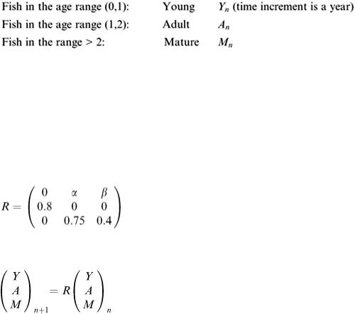
Suppose there are three categories of fish:
where say, Y n denotes the number of young fish (in hundreds) in year n. There are survival rates and birth rates to be specified.
Suppose that 80% of Y survive into the next age category A and 75% of A survive into M. In each case here the depletion is taken as due to natural causes of disease and predation. Also suppose that 40% of M survive without dying out from one year to the next.
There are two birth rates to be set: births of young fish from both the other two categories specified here. It is useful to denote the birth rates as parameters α and β since these can be regarded as under control as the model is evaluated. It is convenient to display this data in matrix form:
Taking, say, α = 2 and β = 1 and starting with a population size of ( Y, A, M ) T = (100, 50, 20) T , then a set of simultaneous difference equations is created by expanding the matrix equation
to give:
The matrix R is known as a Leslie matrix (see Leslie, P.H. (1945) Biometrika, vol. 33, 183–212). Note that the use of difference equations in mathematical modelling is given full treatment in chapter 5 of this book.
The birth rate choice α = 2 will mean for instance that ‘for every one hundred adult salmon there will be two hundred young born each year’. The validity of this data can be checked.
A simple ‘click and drag’ operation on a spreadsheet (or any alternative calculation procedure) will show that after 10 years ( Y 10, A 10, M 10 ) T = (2840, 1575, 1084) and still growing.
Clearly taking larger values for α and/or β will merely accelerate the ‘blow-up’.
It appears that no steady state can occur, but possible values for the parameters α and β can be sought so that a steady state will exist. Mathematically the steady-state requirement means that we want the constant vector
 obtained by considering
  for large n
This requires the solution of the homogeneous set of linear equations:
Simple elimination produces the condition: 0.8α + β = 1, remembering that the trivial solution ( Y, A, M ) T = (0, 0, 0) T is rejected.
This condition provides a line of feasible birth rates, as indicated on the graph in Figure 2.18.
Selecting say α = 1 then β must = 0.2 (point P) for steady state. This can be tested on the spreadsheet and convergence is verified to ( Y, A, M ) T = (73, 58, 73) T , from the same initial population choice. Other values of α and β can be tried.
This initial model does not contain harvesting, so we introduce this as follows. Assume that only the categories Adult and Mature are harvested and that a certain proportion of each are removed each year. Suppose that these proportions are denoted by p A and p M respectively. Thus going forward in the original model we now have
(2.22)
where H is the harvesting matrix 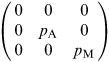 and I the third-order unit matrix.
This model can again be investigated for potential steady state. Substituting the same survival data as

before, but retaining α and β in the equations gives the system for steady state:
(2.23)
This is again a homogeneous system of equations for which a non-trivial solution is required. After a little manipulation, the condition for non-trivial ( Y, A, M ) T is:
This is the ‘big’ equation for the fish farmer. Unless his harvesting policy results in this being satisfied, the model predicts his business will crash in some way or other. To examine the outcome, the values of α and β can be chosen as α = 1.2 and β = 1. The condition then reduces to the form:
Figure 2.18
(2.24)
Recalling that the quantities p A and p M are proportions and so lie in the interval 0 ≤ p A , p M ≤ 1.0, then a graph of feasibility can again be constructed as shown in Figure 2.19 (this time a curve).
This output is easily generated from a spreadsheet graphing facility. Interpretation
Referring to Figure 2.19, this gives a ready-reckoner for the farmer to choose the harvesting proportions. Its particular position obviously depends on the survival and birth data. There is an important further point to consider: what proportions of Adult and Mature fish should be harvested in order to gain maximum profit?
This question can be investigated if some notional price is assigned to the two harvested categories. For greatest profit, then sale of the greatest number of fish at the higher price should be advocated. But from reference to Figure 2.19 it is seen that the maximum permitted p A value is 0.490 and the maximum permitted p M value is 0.935. Thus there is a restriction on Adult fish harvesting of some severity as less than half of this category can be removed each year. Ideally the steady-state line needs to be moved up a bit, more towards the top right-hand corner which would correspond to high values for both p A and p M . There is scope for experimentation with the given data. The question arises, of
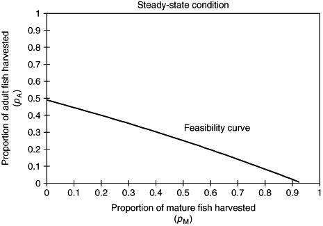
Figure 2.19
course, ‘how many fish do we actually have anyway?’ The answer to this (in the steady-state situation) is to solve the homogeneous set (equation 2.23), which will not, of course, be fully determined.
To illustrate the harvesting and sale problem, let us suppose that p M = 0.5, which implies from equation (2.24) that p A = 0.249, α and β having already been chosen. This data is substituted into equation (2.23) and the solution obtained is ( Y, A, M ) T = c (80, 64, 45) T , where c is an undetermined multiplier. The fact that the solution is not completely determined does not thwart the investigation, however, since we can speculate that the entire farm has a holding capacity of, say, about 20,000 fish. Taking c = 100 gives the steady-state categories held at (8000, 6400, 4500) accounting for a farm holding 18,900 fish.
This means that each year, 1600 Adult and 2250 Mature fish are sold. A spreadsheet graph of the outcome is shown in Figure 2.20 as the steady state is reached.
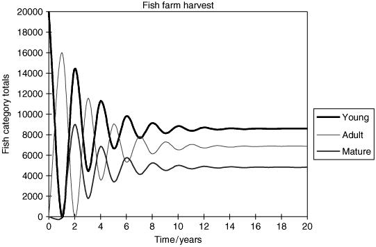
Figure 2.20
Example 2.8 Student loan finance
Affording a place to study at university concerns all potential students. There may be fees to pay for the courses and there will certainly be a need for finance for cost-of-living expenses. Many students take up part-time employment whilst at university, sometimes working during term time as well as
vacations. Support agencies offer help in a variety of ways with scholarships and bursaries, and fees may be means-tested or perhaps not be charged at all in certain countries. Currently a Student Loans Company (established in the UK in 1990) can provide the maintenance aspect of student finance. In this case the company will loan students a given sum at the beginning of each of the three or four academic sessions covering the duration of the degree course. Repayment of the loan will start when the graduate is in work and earning above a certain (cut-off) salary. Essentially the financial package is calculated in the same manner as other forms of borrowing in which a loan gains interest, which is compounded on the original principal sum borrowed, and a repayment amount is set so that the amount owed gradually reduces.
Problem description
It is convenient to investigate the finance of a straightforward repayment loan as a starter model here. This allows the principles of the compound interest effect to be understood and also allows another simple application for ‘spreadsheet modelling’ to be demonstrated. Students can borrow upwards from £2000 per annum from the Student Loan Company, so it is illustrative if we examine the implications of say a £8000 loan debt to be paid off once the student is in employment. Repayments are collected through National Insurance Contributions in the UK and the amount repaid by an individual depends on marginal income earned above the cut-off. Currently repayments are calculated at 9% per annum of marginal income. In this way the amount repaid will increase with the greater annual salary earned by the graduate. The ‘straightforward’ loan repayment system on the other hand is worked out on the basis of a constant sum repaid per time unit with a fixed interest rate charged on the amount outstanding by

the loan authority. Many variations on the same theme can be investigated from a resulting spreadsheet model.
Model formulation
We realise that the development of a generic formula for loan repayment is the first objective. This implies that a variable list should be drawn up to identify the key quantities – see Table 2.11.
Notice that the time period is listed in months here. For situations such as mortgages the time unit will usually be in years, but repayments are still evaluated per month.
The model formula is now built up on a month-by-month basis. A simple line diagram helps to identify the situation – see Figure 2.21.
Table 2.11 Loan repayment variables
Figure 2.21
At the end of each month the amount left to pay is equivalent to the previous month's total plus interest minus one payment. This means that after month one, the amount left to pay is
At the end of month two this amount is
Similarly at the end of month three this amount is
This equation can be rearranged to give on the RHS:
It follows that after n months the amount left to pay would be
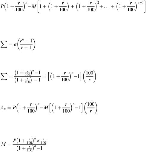
The part of this formula contained within the square brackets is a standard geometric series with an
increasing factor of  . The sum of such a series is calculated using the well-known GP series sum formula:
We can apply this formula by substituting the values a and r as 1 and  respectively. The equation then becomes
If this formula is substituted into the repayment formula in place of the geometric series then the repayment formula becomes
(2.25)
This gives the amount outstanding at the end of n months.
Since this formula equals zero when payment is complete after N months it can be rearranged as follows to calculate the monthly payment M:
(2.26)
Interpretation
A table of the month-by-month account is usually needed by the borrower. This is easily provided by setting up the spreadsheet as shown in Figure 2.22. Data has been selected for illustration: P = 8000, r = 0.25, N = 60.
Calculation from equation (2.26) gives that monthly repayments are M = £ 143.75. The spreadsheet shows the calculation for the first 12 months.
The spreadsheet output and formulae are shown in Figure 2.22 so that the model implementation can be easily understood. The amount owed A n in total after month n can seem slow to reduce. If this is graphed as a function of n, its non-linear ‘concave downwards’ shape can be clearly displayed as shown in Figure 2.23.
In Figure 2.23 we have accentuated the concavity for illustration by increasing the rate of interest r suitably. There are plenty of ‘What-if’ questions that can be answered directly from the spreadsheet model by simply changing values of the data input, not necessarily when n = 0 but after a certain number of months have elapsed first.
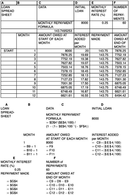
Figure 2.22
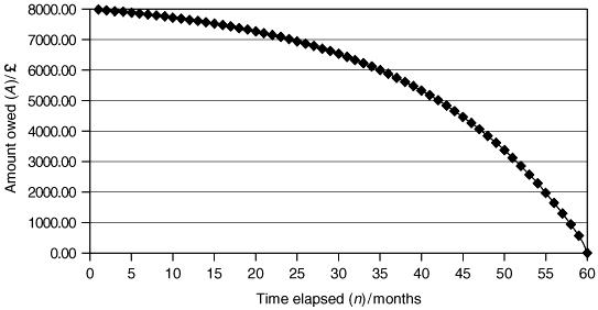
Figure 2.23
Example 2.9 Car exhaust bay
For the next example we shall introduce a random effect into the model building. By doing this a very important area of mathematical modelling can be given prominence at this early stage in the text. Experienced modellers recognise the difference between ‘deterministic’ models and ‘stochastic’ models and it is the latter category that we will dip into here for a brief introduction. Another example follows as Example 2.12. To immediately see what is involved let us imagine the situation at a small garage, which has a one-bay facility for instant replacement of vehicle exhaust and silencer systems. What happens is that cars arrive with some fault that requires immediate attention, normally the fitting of a new part. The service time will vary depending on the amount of wear on the exhaust, so other drivers arriving may perhaps move on to another garage. The modelling problem is concerned with how the garage copes with demand over a representative time period. The decision on this matter ‘cuts both ways’ since drivers do not want to wait before getting their repair, whilst on the other hand the garage do not want staff hanging around with no job to do. The random effect referred to concerns the fact that we do not know in advance when cars will turn up and also we do not know the length of time necessary to effect a repair. This does not prevent a useful model being formulated, however, based on data collection and use of theoretical statistical distributions.
Problem description
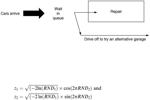
There are two ‘random’ events to deal with in what has been outlined above – arrivals of cars and subsequent repair times. The situation can be displayed in the diagram shown in Figure 2.24 for clarity.
A common feature of modelling problems of this kind is that queues can occur in the system leading to a delay and decision from ‘customers’ on whether to bother to wait. Arrival times of the customers will be random as also will the service time. In our garage problem the customers are the car drivers and the service time is the time required for the repair to be undertaken. The outcome from the model will be a little different from that encountered in the earlier examples in this chapter. Instead of a single numeric answer or a set of determined results, here we are seeking answers to questions such as ‘can the garage cope adequately with the demand for repairs?’ or ‘what is the average daily percentage of potential customers that decide to take their business elsewhere?’ The model will require car arrival times to be generated from a stream of random numbers and by continually changing the random number stream
we get many simulations of the repair process (in the simplified case illustrated in Figure 2.24). It is from a series of simulations of the same event that we can calculate averages of waiting times and so on.
Model formulation
The two effects in the simple garage situation have to be modelled. The best method would be to attend a typical garage and observe what happens in practice: gather data on arrival times (more particularly inter-arrival times) and throughput times for the fitting of a new exhaust. The data would then be assembled and its pattern examined for statistical representation. For this first example of a random number model it is more instructive to make statistical assumptions a priori about the nature of the arrival times and repair times. We shall suppose that:
Figure 2.24
1.Inter-arrival times follow an exponential distribution and so can be modelled by the formula – m ln( RND ) where m in the average inter-arrival time and RND is a random number.
2.Service times follow the normal distribution N (μ, σ 2 ), characterised by the values for the mean (μ) and variance (σ 2 ). Two variates of the standard normal distribution are then produced by taking two RND values and calculating:
These can be converted for N (μ, σ 2 ) by calculating σ z 1 + μ and σ z 2 + μ. (See Chapter 7 for details of the statistical theory that underpins these techniques.)
To set up the model it is only necessary now to state values for the parameters m, μ and σ 2 . We can then draw on a stream of random numbers and set up the effect on a spreadsheet. There is also the waiting time question; for simplicity here we stipulate that if on arrival of a customer the service facility is already in use, then immediately drivers move on to another garage. Thus this is now reduced to a simple situation, not probably truly representative of real car exhaust repair firms where there are usually four or five separate repair bays, many operatives, and customers may be content to wait a considerable time if they feel assured of getting a reliable job done. Nevertheless at the beginner stage it is useful to get the hang of simulation modelling of this type.
As stated, three parameters are to be chosen. We will take m = 30 min = 0.5 hour, μ = 0.75 hour and the standard deviation for service times, σ = 0.25 hour. These seem reasonable trial values and because the service time is longer than the inter-arrival time, then we might expect a queue to build up. The resulting spreadsheet is shown in Figure 2.25 and its construction is a useful exercise in its own right since there are some decision outcomes to include. The numeric output of a typical spreadsheet model for this example is given in Figure 2.25, followed by the ‘formula’ version (Figure 2.26) which drives the spreadsheet calculations. The data refer to the first 12 driver customers.

The spreadsheet is 12 columns in width to include up to the decision: does the customer get served or immediately depart. This may seem at first glance a simple question since the answer is ‘if a customer is already being served occupying the repair bay, then drive off, otherwise get immediate service’. However, to automate this on a spreadsheet requires some logical statements to be included, in columns K and L. The procedure is best explained by tabulating the spreadsheet formulae:
It can be seen how the logic is organised using the ‘ IF ’ statement, which is a common feature of spreadsheet capability. In most spreadsheet programs this statement is:
There is a nesting facility so that the outcome in say the second parameter can be a further IF statement. Spreadsheet logic includes the use of AND, OR and NOT.
To see how the IF statement works in the garage example, refer to the entries in the columns K and L. What we are trying to achieve in the cells shown is the decision whether the next car arrival can be served. This is obviously determined whether a customer is already occupying the repair bay. To convert this simple decision into a spreadsheet logical statement requires a little thought. We must keep account of the expected finishing time of the current car being serviced, remembering that some drivers may have already been turned away. To begin with and shown here we want to know whether the next arrival will ‘leave’ or be ‘served’ – hence the style of the IF statements.
[It should be noted that in this spreadsheet detail, the evaluations begin in row 9, hence the reference to cells E9, J9, K10 etc.] The successful account of who is served and who is not can be seen in the output in Figure 2.25. The spreadsheet formulae in the earlier columns can easily be seen as the construction of the arrival times of cars and the simulation of the service times required.
Interpretation
By counting up the results of the first 12 drivers to arrive, it is seen that five are served and seven leave for service elsewhere. The model shown here may now be re-run over different random number streams to simulate the performance over as many days as is necessary for the outcome to be assessed. The model as shown can be improved to show clock times in hours and minutes and to account for the closing of the service after say 5.00 p.m. Other data can be recorded, of course, which will be of use to the garage manager, for example the length of time that the repair mechanic is idle. In reality drivers would not always drive away immediately but may be content to wait for a certain time; also in most locations where car exhausts are replaced, there will be three or four repair bays provided. To include these features in the spreadsheet will need some extension from what has been given here, particularly to keep check on the various queues. For more complex modelling problems of this kind there are commercial software packages available.
Example 2.10 Fixtures
For the next introductory example, we turn to an organisational problem that is quite common in its various forms. The most interesting is the construction of a fixture list for a league of teams from the world of football in which within the league every team is to ‘play’ every other team once at least (and often twice on a home and away basis) to complete the league competition. Such a fixture
Figure 2.25
Figure 2.26
list can, of course, be needed in many other sports and games besides football. The organisation required is pinpointed by the usual need to involve each team in having a fixture on a given day. Organisational problems are encountered elsewhere in everyday life and throw up interesting problems for modellers to solve: for instance in drawing up train and bus timetables, particularly, say, the situation on single track railway where two-way traffic takes place. We shall concentrate here on football fixtures, which provide a good test for our problem-solving ability.
Problem description
In the usual way a particular problem is defined. Suppose there is an eight-team league for which a complete fixture list is required. We can think of this as a football league so that each team is to play against every other team twice, home and away. There is also the requirement that on a particular Saturday (say) all of the teams have a fixture. At first sight this may seem to be a simple straightforward problem, but a moment's thought tells us that a haphazard approach is unlikely to work. It should be noticed that in many of the Getting Started examples a certain number of assumptions are often needed to help develop a mathematical model. In the fixture case there does not appear to be any assumptions and it is true that the problem as set can be immediately tackled. However, referring to the
football scene, we must appreciate that each team wants an even spread of home and away games. Also there may be rivalries between local team where special attention is needed to the fixture order (perhaps also two teams share the same stadium). The way forward is nevertheless to first tackle the eight-team league situation. Note finally that whereas in earlier examples the model formulated has often ended up as an equation to be analysed, here the outcome is the complete set of fixtures.
Model formulation
Denote the eight teams by A, B, C, D, E, F, G and H. A particular sequence of games on the first Saturday is:
1.A v. B
2.C v. D
3.E v. F
4.G v. H
Here we have teams A, C, E and G playing ‘at home’. The following week it is expected that B, D, F and H will appear in the left-hand column indicating a home game. We could therefore merely reverse the games for the second
Saturday programme, but this may not be sensible (why?) so a permutation of the away sides can be carried out. The fixtures could be continued in this way, but it should be quickly clear that this development confines A, C, E and G to one column and B, D, F and H to the other so that we will not achieve the required result.
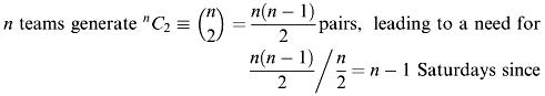
It is worth considering how many games are to be played in total and therefore how many ‘Saturdays’ will be used up over the complete ‘season’. For the eight teams a fixture is the pairing of any two
teams. This can be done in  ways. This evaluates to 28 ways or 28 games in all, before allowing for ‘home’ and ‘away’. Thus our eight-team league needs a total of 56 games which takes up 14 Saturdays since there will be four fixtures each Saturday. The number of Saturdays spans about three months only, so if we wish to fill up the entire winter with football then there is clearly spare capacity. On the other hand for cases where there are more teams in the league it can be seen that the number of fixtures expands:
there are n /2 games each Saturday. This will be 2( n − 1) Saturdays when ‘home’ and ‘away’ are taken into account.
These are important preliminaries for the fixture devisor to contemplate.
To return to the main task of constructing the fixture list. We now know that for an eight-team league, there are seven different sets of, say, weekly fixtures, repeated to give a total of 14 Saturdays. The best way to solve the problem is to fill out a game matrix as shown in Figure 2.27.
Examination of the pattern in the ‘matrix’ shows how the fixtures can be developed. Starting with team A, we give it the fixture list versus B, C, … H, without loss of generality. For team B, start two rows lower down and give it the fixtures C, D, … G.
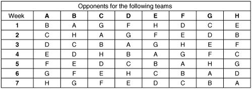
Its first game is versus A so the remaining game in Week 2 is versus H. Now consider team C: again start two rows further down and roll to alphabetical list round into Week 1 as necessary. Vacant weeks are filled in by reference to what has already been decided for team's A and B. By continuing in this way it is easy to complete the entire schedule.
This method is easy to extend to 10, 12 teams and so on. Interpretation
To see what the fixture matrix has delivered, write down the games allotted for the first two weeks: Week 1 (A, B) (C, G) (D, F) (E, H)
Week 2 (A, C) (B, H) (D, G) (E, F)
Writing the games down in pairs allows for suitable selection of the home team. We would continue for subsequent weeks in the same manner until the first seven weeks are complete. The remaining seven weeks’ fixtures are merely the reverse of the first seven weeks.
This is not quite the end of the problem for a particular real situation if allowance is to be made for ground sharing or avoidable fixture juxtaposition. This new problem can be easily fixed since there is complete flexibility in the matrix fixture outcome, however, weeks can be interchanged and of course the team letters A, B …. re-assigned. A further situation that might cause a difficulty is if there is an odd number of teams.
There are other fixture situations that occur commonly. For example a mixed-doubles tennis tournament played out all on one day on say two courts where all of the pairs play one another. Given that there are six pairs entering, what is the order of play so that couples get a reasonable spread of games and rest? Then there is the club badminton match in which three pairs from Club 1 play all the three pairs from Club 2, all games on the one church-hall court in one evening: what is the order of play?
Figure 2.27
Example 2.11 Snow plough Problem description
On the occasions when there is a sudden very heavy snowfall, country roads can easily become blocked. This necessitates the use of the local council's snowplough in order to clear a way through. In a particular situation a long 10 km stretch of road has to be cleared after a fall that results in an even depth of 0.5 m along the road. The clearance would be routine at a steady slow pace
apart from the fact that, just as the snowplough is about to move off, it begins to snow again heavily. As
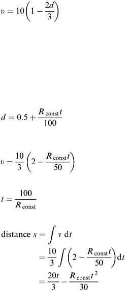
the depth of snow increases, so the speed of the snowplough decreases until, at a certain depth, the snowplough itself can get stuck.
The rate of fall of the new snow will affect the progress of the snowplough and the question that arises is whether the snowplough can complete the 10 km clearance or find that the snow builds up so quickly that the snowplough gets stuck.
We shall consider the following data.
1.It snows for 1 h in total.
2.The snowfall rate may vary, but at its heaviest it is 0.1 cm s −1 .
3.The snowplough gets stuck when the depth of snow reaches 1.5 m.
4.On a road completely clear of snow, the plough travels at 10 m s −1 . Model formulation
To make a start, let us suppose that the speed v of the plough decreases in direct proportion to the depth d of snow. Measuring v in metres per second and d in metres, we arrive at the formula
(2.27)
valid for d ≤ 1.5, after which the snowplough has stopped. Other relations can be constructed for calculating the speed in terms of the depth of snow, but this is the most simple. Note that this relation satisfies the data given: v = 10 when d = 0 and v = 0 when d = 1.5. Also using equation (2.27), since the initial depth of snow is 0.5 m, the plough moves off on its journey at 6.7 m s −1 .
Now the new snowfall rate has to be modelled by a suitable function. Earlier we said that the rate can vary throughout the hour of the fall. However, to make the model simple to begin with, suppose that the snowfall rate is taken as constant. Denote this by R const (cm s −1 ). Therefore the increase in depth of snow is R const t cm = R const t /100 m in t s. The total snow depth now is
(2.28)
This enables the speed of the plough after t s to be obtained by substituting from equation (2.28) into equation (2.27), giving
(2.29)
If v has declined to zero, then the plough has stopped, and this occurs when (2.30)
The distance travelled in this time by the snowplough will be obtained by integration:
(2.31)
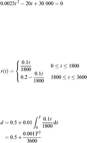
(Remember that s = 0 initially.)
Now try some data to see what happens.
Case A Suppose that a heavy snowfall takes place at the maximum rate of 0.1 cm s −1 . If snow continued to fall at this rate for the entire hour, then the extra depth of 0.1 × 3600/100 m = 3.6 m would accrue on top of the original 0.5 m, which is very unlikely. However, before rejecting this forecast, we shall see what has happened to the snowplough by using equations (2.30) and (2.31).
From equation (2.30), the plough stops when t = 100/0.1 s = 1000 s = 16.67 min.
From equation (2.31), we can work out that the plough has travelled a distance of 20 × 1000/3 − 0.1 × (1000) 2 /30 m  3333.33 m = 3.33 km. So the plough travels exactly a third of the way along the road before getting stuck. The depth of snow at this moment is obviously 1.5 m, which is a long way short of the projected final depth of 4.1 m after 1 h. However, once the plough has stopped, it remains stuck until further relief is available; so it may as well now stopsnowing!
Case B Suppose now that a less heavy snowfall takes place at a steady rate of 0.025 cm s −1 . This time, from equation (2.30), the plough comes to rest after 100/0.025 = 4000 s  66.67 min, which of course is four times as long as in Case A. The distance travelled in that time is again worked out from equation (2.31) as 20 × 4000/3 − 0.025 × (4000) 2 /30 m
  13 333.33 m = 13.33 km. However, this is further than the allotted 10 km on the road to be cleared; so we conclude that the snowplough has achieved its target, assuming another plough has responsibility for the additional road. The actual clearance time can be worked out by substituting into equation (2.31) that s = 10 × 1000 and R const = 0.025. The resulting equation can be reduced to
The solution that we want from this is t = 2000 s  33.33 min.
The speed of the plough after 10 km can be calculated to be 3.33 m s −1 by substituting into equation (2.29).
Finally, we shall consider a situation where the new snowfall rate is not constant. Suppose that the rate increases steadily up to the maximum rate of 0.1 cm s −1 after 30 min before decreasing again. The snow rate profile is shown in Figure 2.28.
Denoting the rate by r(t) cm s −1, then
The calculation of the depth of snow follows by integrating the expression for r(t). The technique needs a little care owing to the nature of r(t) where we have defined it by a different function over the separate time ranges.
For current time T ≤ 30 min,
(2.32)
This gives a depth of snow of 1.4 m after ½h. For current time T > 30 min,
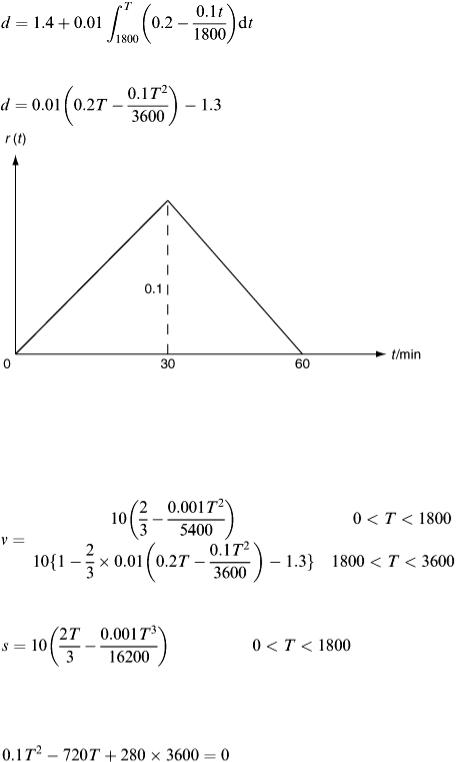
After a little simplification, this reduces to
(2.33)
Figure 2.28
At the end of an hour, the depth of uncleared snow can be calculated by substituting T = 3600 into equation (2.33). This gives a final uncleared depth of 2.3 m.
We must now return to equation (2.27) to obtain the expression for the speed of the plough. The results are.
and by integration
This means that after 30 min, the plough has travelled 8.4 km and its speed is 0.67 m s −1 . The snow is 1.4 m deep at this point so clearance continues, but not for long. Setting v = 0 gives a quadratic for the time T :
which has a root at T = 1903, i.e. after another 103 s the plough gets stuck. The additional distance travelled is about 34 m.
Interpretation
The results seem correct for the data used. Other situations can be analysed. An interesting further question concerns what is happening behind the snowplough. Immediately behind the plough the road is clear, but further back it is snowing and the depth is building up again. If the snow depth profile were
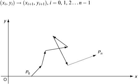
photographed after say 30 min what would the picture show? Example 2.12
Random walk
To conclude the set of examples that illustrate simple modelling problems, we return to a situation involving simulation modelling with a random effect to be taken into account. Example 2.9 examined a queue scene (the start of many operational research investigations incidentally). Here we take up a different problem involving a random walk. This examines the path of a single point in two dimensions in which a walk takes place over say the n straight-line segments:
This can be drawn out as shown in Figure 2.29.
Figure 2.29
The random part of the procedure is that from any given point P i ( x i , y i ) in the walk to the next point P i +1 the distance and direction are randomised. The outcome is then indicated on Figure 2.29, showing n steps from P 0 to P n . When the procedure is repeated over a different set of random numbers, a different path will be executed.
This implementation may seem a little esoteric and have little relevance to mathematical modelling. However, this is very much not the case and we don't rely merely on the supposed real-life situation of the drunken man trying to walk home from the public bar after a night out! Random walks (or growth) can be used to model, for instance, dirt collection and organism growth. In the case of dirt collection, this is important in many industrial processes leading to a foul up of the operation when for example the ‘cogs’ jam. Modellers are called in to help predict dirt build up in which small particles gather in some random manner in machinery. In the case of organism growth, we can turn to the spread of fungus through the growth of small spores from some initial source. It will be important to predict how fast the fungal growth spreads. The spores can be taken as a random spread from the source. These two situations are really three dimensional of course so by displaying a planar walk in Figure 2.29 we are thinking more of the drunkard than the scientific applications.
It may be thought that in this example we are extending the simple modelling tasks beyond that suitable for beginners, but remember all the examples start from a real-life problem that can be modelled usefully by students on an initial modelling course since we reduce each problem to a core activity within the scope of beginners.
Problem description
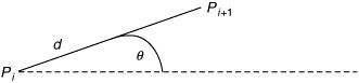
Consider a simplified version of White Rot Fungi spread from a tree trunk subject to a suitable damp environment. Suppose that the trunk is infested with
the fungal source and that this is represented mathematically by a set of source points along a line of the trunk. Again a two-dimensional case will be analysed for simplicity and, in order to suitably calibrate the fungi spread, let us suppose that a line of tree trunk can be represented by the x axis and that the fungal growth is away from the tree ( x axis) in the positive y direction. We need to set up a random walk starting at a number of points along the x axis. Each spore line will have a random length and a random direction subject to what the growth behaviour is likely to be.
Model formulation
The real dimensions of the problem are required so that the correct behaviour can be reflected by the model. However, to illustrate what can be formulated, it is convenient to use ‘dimensionless’ problem units for simplicity. Taking the random walk path of one given starting point on the tree trunk, then the path indicated in Figure 2.29 needs to be modelled. The path from P i to P i +1, i.e. ( x i, y i ) → ( x i +1, y i +1 ) can be shown in Figure 2.30.
The two parameters d and θ determine the position of the point P i +1 starting from P i . These require attention to be converted into random variables.
1.Taking d : suppose this variable is normally distributed with mean of zero and standard deviation of 1.0.
2.Taking θ: suppose this is a uniform random variable over the range (0, π).
These decisions will allow the spore growth to be ‘backwards’ towards the x axis base line so when the outcome is put onto the computer we must take account to prevent growth back into the tree itself.
The situation is best developed using the MATLAB package (The MATH WORKS Inc., Natick, MA, USA). MATLAB is a user friendly compiled programming language ideal for modelling simple transient problems of the kind considered here. When MATLAB is run for a case where there are four neighbouring source points for P 0, then the outcome is easily graphed as shown in Figure 2.31.
Figure 2.31 shows the growth away from four source points which have representational coordinates (1,0), (2,0), (3,0) and (4,0) and is taken over two
Figure 2.30
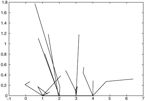
Figure 2.31
time steps for illustration purposes. When we continue with the simulation to cover the first 10 steps then we can view the consequences as shown in Figure 2.32.
This looks more like the sort of scrambled growth pattern to be expected. Each spore has 10 growth steps (unless suppressed by ‘hitting’ the x axis). The MATLAB program code for this is given at the end of this chapter (Appendix 2). As in any simulation model it will be necessary to run over many different random number streams so that average effect can be assessed.
Interpretation
We can immediately see the potential of random walk models in representing the fungal growth. The spore lines overlap and are congested close into the tree trunk. There are questions we can answer mathematically from the simulation, which it is then hoped will be useful to the environmentalist. For example:
1.Measure the density of lines against the distance away from the base line.
2.Measure the greatest extremity of a spore for a given number of time steps.
The model can be easily changed if it is decided that the random variables used need adjustment. We can compare our outcome with photographs of the real thing. The nature of the investigation can also be re-constructed if the growth of fungus out from a circular cross-section of tree is required.