Figure 6.11

A length of chain is hanging over the edge of a horizontal deck. The weight of the part hanging vertically down causes the whole length

6.9 to slide off. Motion is slowed by the friction between the chain and the deck. Formulate a mathematical model to predict the motion of the chain.

6.4 Second order, two variables (uncoupled)

When a body moves in two dimensions, we need two coordinates to specify its position at a given time. Effectively we apply Newton's second law in two directions to obtain two equations of motion. Usually these equations are uncoupled in the sense that each coordinate variable appears in only one equation. The resulting mathematical formulation will be two simultaneous second-order differential equations. Examples of this situation occur when we are modelling projectile motion. As an example which contains features a little different from the standard projectile, consider the following ‘fireman’ problem.

Example 6.4 Context

A fireman is directing a jet of water into a window of a burning building. Owing to the heat, and the danger of a wall's collapsing, the fireman wishes to stand as far back as possible, while still being able to direct the water jet through the window. The scene is illustrated in Figure 6.12.

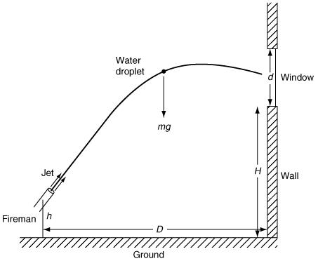
Figure 6.12 Problem statement

In mathematical terms, the problem objective is to find the maximum value of the distance D so that the jet still reaches the window.

Formulate a mathematical model

Some of the quantities in Table 6.4 are more important than others. Depending on the sophistication of the model, we may decide to ignore certain features. To make a start, some assumptions are listed as follows.

1.The water jet is effectively a stream of particles.

2.We can neglect air resistance, cross-winds, change in water pressure, etc.

3.The size of the window is neglected in the first model.

It is convenient to draw another diagram (Figure 6.13) in which the forces and velocities can be shown.

As we have hinted at the start of this section, we need to obtain two equations of motion. One of these will represent the horizontal motion and the other the vertical motion. Newton's second law can be applied in each direction separately and, in doing so, we get a pair of uncoupled equations, i.e. the dependent

Table 6.4

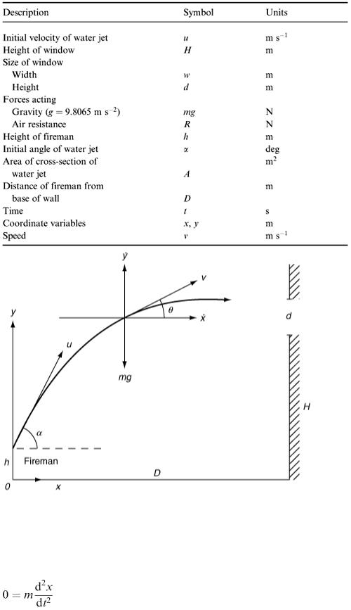
Figure 6.13

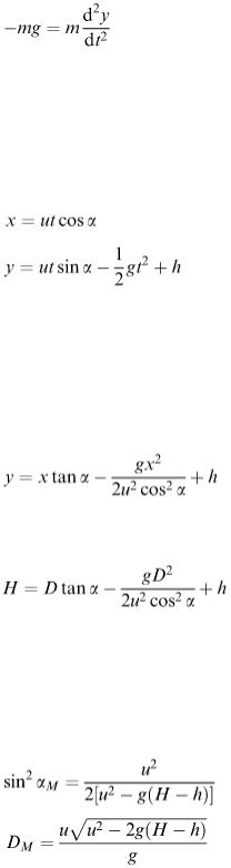
variables do not appear in both equations. This uncoupledness will help us to obtain the solution to the model. In the next section, we see a situation where the model involves coupled differential equations with a resulting different approach to the solution. Remembering that Newton's second law states that force = mass × acceleration, we now apply this law to get our two equations: for horizontal motion

(6.10)

and, for vertical motion,

(6.11)

Note that we have inserted m into the equations without saying what m represents. We can imagine a small group of droplets sufficiently close to be taken together as a particle of mass m. The jet of water can be regarded as a stream of such particles. The point about uncoupledness can be seen in equations (6.10) and (6.11) since the dependent variables are x and y.

Obtain the mathematical solution

Two straightforward integrations of these simple ordinary differential equations give (6.12)

(6.13)

(do not forget the height of the fireman which is h ).

This is nice and familiar, but what are we supposed to be trying to solve? This was how far away the fireman can stand and still direct his jet through the window. A moment's thought tells us that we are not really interested in how long it takes for the water to reach its destination but are concerned with the distances and angles involved. (Anyone in a burning building wishing to be rescued certainly will be interested in how long the water takes to arrive, but that is rather different.) So, if time t is eliminated between equations (6.12) and (6.13), then

This equation applies to all points on the jet. In particular, taking the jet to pass through the point x = D, y = H (corresponding to the bottom of the window), then

(6.14)

Now what interpretation do we put on this equation? On reflection we realise that H, h, g and u are fixed, so that D is the variable to be maximised over changing α. Regarding α as a continuous variable, we can differentiate in the usual way and put d D /dα = 0.

This results in the condition u 2 / g = D M tan α M , where D M and α M are the optimum values sought. After some manipulation, we arrive at the equations that we want as the mathematical solution of the model:

(6.15)

(6.16)

Note that equation (6.16) is valid only for u 2 > 2 g ( H − h ). Why do you think this condition is necessary?

Interpret the solution

Can this result be validated? The following data are supplied and are substituted into equations (6.15) and (6.16). Given that u = 20 m s −1 , h = 1.5 m and H = 15 m, then it is easy to calculate D and α to

get D M = 23.7 m and α = 59.8°. Using the model

This model is capable of further development since there are several factors that we have neglected or not investigated which might affect the usefulness of the results.

1.At what angle does the water jet enter the window?

2.The size of the window has not been brought into the model.

3.How sensitive are the results to changes in u, h and H ?

4.A water jet will spread out as it travels from the pipe; can we say anything about this spread?

5.Air resistance acting on the water flow has been ignored—was this justified?

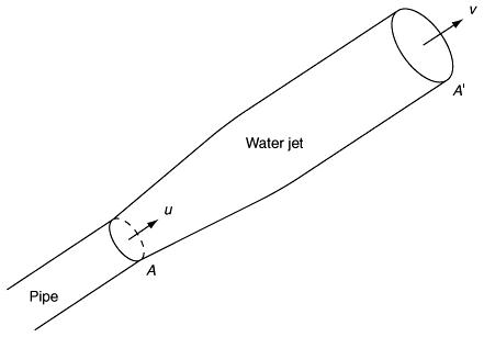
The modifications necessary to deal with all these situations are left for you to incorporate, but we can see that (b), for example, will affect the validity of equation (6.14) since it is not necessary for the water jet to pass through the ‘coordinate’ point ( D, H ). The spread of the water jet is actually easy to quantify by considering ‘mass conservation’ in Figure 6.14.

As the cross-section of pipe is A (m) and the initial velocity of the water jet is u (m s −1 ), the initial volume flow equals uA (m 3 s −1 ). If at some subsequent stage the velocity is v with cross-section A ′, then by the conservation of mass we have uA = vA ′. Taking the diameter of the pipe held by the fireman to be 10 cm, then since u = 20(m s −1 ) we have vA ′ = 0.157. Thus, if v is calculated at some point, in particular as the water is about to enter the window, then we can say something about the spread (do you think that the jet is still circular in its cross-section?). On the assumption that the fireman wishes to get all the water into the open window, this analysis will reduce the variation in D consistent with hitting the target.

Figure 6.14

Exercises

There are a number of modelling problems involving throwing, each of which can be tackled using a similar mathematical model to that used in Example 6.4. Sports and games are a rich source for such investigations and we shall give three situations here.