

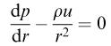
is dimensionally correct, where p is pressure, ρ is density and u is velocity.
The velocity u of propagation of deep ocean waves is a function of the wavelength λ, acceleration
4.28g due to gravity and density ρ of the liquid. By assuming that u = k λ a g b ρ c , where k is a dimensionless constant, find the relationship between u, λ, g and ρ.
Summary
In this chapter, we have looked briefly at some of the more important skills involved in mathematical modelling. It should not be regarded as a complete list but as an introductory guide.
Early on in the modelling process, we need to make a list of factors. These include variables, parameters and constants, some of which can be linked together in groups. It is probably a good
4.1idea to make the list longer than necessary to begin with, just to be sure that you have thought of everything. Go through your list, crossing out factors which you think have only a marginal relevance to the problem. Remember that your first model should be as simple as possible. Try to identify inputs and outputs. Devise a suitable notation and keep track of the units.
4.2Think carefully about your assumptions and try to make a complete and accurate list.
4.3Try to identify which variables affect each other and how the relationship can be represented mathematically.
Care is needed when translating verbal statements into mathematical equations. The verbal
4.4statements are often vague so that there are a number of mathematical options. Choose simple forms in preference to complicated ones.
Compare the relative sizes of the terms appearing in your equations (using data if necessary). This
4.5can lead to simplifications without loss of accuracy and also helps to pinpoint areas where more detail is required.
4.6Reduce the number of parameters if you can. This ultimately decreases the amount of computation required.
All variables apart from those which are pure numbers are measured in certain units. It is vital to keep note of these units
4.71. when collecting data,
2.when making your list of factors for your model and
3.when testing your model against data.
The preferred system of units is the SI system but you may need to convert from and to non-SI
units in any particular application.
4.8Any physical quantity has a dimension which is a product of powers of the basic dimensions M, L and T. Check that all the equations in your model are dimensionally consistent.
4.9Dimensional analysis can help in developing models. It shows how certain variables must be grouped together.
4.10Dimensionless groups of variables are often useful in physical models. In particular, they give an indication of the relative importance of various physical influences.
CHAPTER 5
Using Difference Equations
Aims and objectives
In this chapter we discuss models in which variables are represented as mathematical functions of an integer n indicating how many time intervals have passed. Assumptions have to be made about the changes that occur in each time step and the resulting models involve difference equations.
5.1 Introduction
One of the main points of modelling is to predict the future development of a system. A model of the economy, for example, can be used to predict future trends and so provide a basis for policy decisions. Any such model relies on assuming that the rate of change of a variable X is linked to or caused by:
(1) the present value of X
and\or |
(2) previous values of X |
and\or |
(3) values of other variables |
and\or |
(4) the rate of change of other variables |
and\or |
(5) the time, t. |
The relationship that we want to model is the one that describes how X itself varies with time t. There are two very different ways of modelling such a relationship.
1.We could think of X ( t ) as a continuous function of continuous time t. In this case the graph of X against t would show some continuous curve and our modelling objective would be to write an explicit formula for X ( t ) in terms of t. The way in which X changes with time can in this case be described by a differential equation. We discuss such models in chapter 6.
2.We could think about values of X only at particular points in time, for example at intervals of one hour or once a month. In this case we use a symbol such as X n to denote the value of X after n intervals of time have passed ( n is referred to as a ‘subscript’). A plot of X n against n is now a set of separated points rather than a curve and we call this a discrete model.
The way in which X changes with time can now be described by a difference equation.
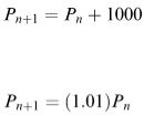
Suppose the population of a town increases by 1000 every year. Using P n to denote the population after n years, a discrete model describing how this town's population increases is:
Suppose instead, that the population increases by 1% every year. In this case the appropriate model would be:
A population with a net growth rate (births – deaths) of 2% p.a. and a net annual immigration of 100
individuals could be modelled by:
These are simple examples of difference equations.
Solving a difference equation means finding an explicit expression for X n in terms of n and initial values such as X 0 . Note, however, that this can be rather a difficult task and not strictly essential because a model in the form of a difference equation can be used without knowing the mathematical solution of the equation. This is because if we know present and previous values of X we can always use the difference equation to generate the next value, followed by as many values as we like. Of course, the advantage of having a formula for X n in terms of n is that we can substitute any value of n we like into the formula to get an immediate answer.
Difference equations are easiest to solve when they are homogeneous. This means that the equation can be satisfied by making all the X S = 0. For example the equation X n +2 − 3 X n +1 + X n = 0 is homogeneous, while X n +1 − 2 X n = 3 n + 1 is not. It also makes things easier if the coefficients are constants. For example, X n +2 − 3 X n +1 + X n = 0 has constant coefficients while X n +2 − 3 nX n +1 + X n = 0 does not.
Mathematical methods for obtaining solutions of difference equations can be found in many textbooks (see the Bibliography for examples) and will not be described in this chapter. Here we are only concerned with the formulation of models in terms of difference equations and their possible application.
A difference equation connecting X n +1 and X n and no other X values is called a first-order difference equation. If the equation also involved X n −1 or X n +2 we would call it second order, in other words the order is the difference between the highest and lowest subscripts appearing in the equation. Not surprisingly, first order difference equations are the easiest to deal with. They are also the most useful for building models.
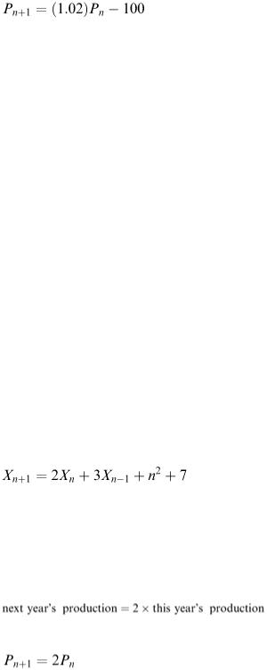
More significant than the order is the question of whether the difference equation is linear. An example of a linear difference equation (this one happens to be second order) is
Note that the presence of the n 2 does not make the equation non-linear, the important thing is that all the X terms are only multiplied by constants.
Example 5.1
Suppose P n represents an industry's production output in year n and that production doubles every year, so that:
that is
If P 0 = production in year 0 then P 1 = 2 P 0 , P 2 = 2 P 1 = 2(2 P 0 ) = 2 2 P 0 and P 3 = 2 P 2 = 2(2 2 P 0 ) = 2 3 P 0 . The pattern is clear, every year we multiply by 2 so after n years we have multiplied by 2 a total of n times, i.e. by 2 n . Another way of describing it is to say that the P values are going up in a geometric progression and the general solution is P n = 2 n P 0 . A similar equation applies whenever the growth rate is a constant percentage, for example if the growth rate is 25% per annum then the difference equation is P n +1 = (1.25) P n and the solution is P n = (1.25) n P 0 . This kind of situation is
very common with investments where interest accumulates at a constant r % per annum. If P 0 is the initial amount of money invested, the amount P n after n years satisfies the equation P n +1 = (1 + r / 100) P n and the solution is P n = (1 + r /100) n P 0 .
These are all examples of the difference equation X n +1 = aX n which corresponds to the assumption that a variable increases in a fixed ratio (or percentage) in each time step. The solution of this is X n = a n X 0 (as can be verified by changing n into n + 1). The two statements X n +1 = aX n and X n = a n X 0 are in fact equivalent. The first is the difference equation and the second is its solution.
The behaviour of the solution (i.e. the way X n changes with increasing n ) depends on the constant a, which can be thought of as a growth factor. If a > 1 then multiplying X n by a gives a bigger answer so X n +1 > X n and the X n values increase with n. If 0 < a < 1, multiplication by a gives a smaller answer so X n +1 < X n and the X n values continue to decrease, eventually to zero as in Figure 5.1.
Figure 5.1
Negative values of a give a different behaviour because each multiplication by a changes the sign. We therefore get oscillations, decreasing in amplitude if − 1 < a < 0, while the oscillations increase in amplitude if a < − 1 as illustrated in Figure 5.2 (where the points have been connected by lines to help trace the sequences).