


8.4 Estimating parameters
As we saw in chapter 4, our main concern in mathematical modelling is to formulate relationships between variables but these also almost invariably involve parameters. For example,
where x and y are variables, and a and b are parameters. In this general form a model can be of some use in predicting general behaviour in a descriptive fashion, such as ‘when x increases from zero, y increases until x = b /2 a and then decreases, becoming zero at x = b/a’. To use the model in a direct practical way, however, we must obtain numerical values for the parameters and we can only get these from data. The process of using data to obtain parameter values relevant to a particular application of the model is often called ‘calibrating’ or ‘tuning’ the model. The usual methods of obtaining the parameter values are as follows.
1.Graphical.
2.Statistical, usually involving least-squares estimation.
3.Mathematical, usually requiring the solution of linear equations. Example 8.4
In section 8.3, we obtained the empirical model W = 16.78 H 2.3 from the data on 15 people. Without any data, what kind of model could we develop for predicting a person's weight from his or her height?
Solution
A very simple model can be derived by assuming that all human beings are different-sized copies of the same geometric shape and made of the same material. Since weight is proportional to volume (for constant density) and volume is proportional to (height) 3 , the simplest model is W α H 3 . This model predicts W = aH 3 for some value of a. We cannot say anything about the value of the parameter a without data. It would clearly be sensible to use different values of a for males and females.
If the data in Table 8.1 are all that we have, how do we estimate the value of a? Using the graphical approach, we draw the graph of W against H 3 (Figure 8.7) and fit the best straight line that we can through the points, not forgetting that W must be 0 when H = 0; so our line must pass through the point (0, 0). Calculating the slope of the line we find that a  12.3.
12.3.
Using the statistical approach, the regression model y = ax + b (where y = W and x = H ) gives y = 11.1 x + 4.19. This predicts that a person of zero height will weigh 4.19 kg! Least-squares fitting of the more sensible model y = ax is done by choosing the value of a which minimises the sum of squares of the errors S = Σ( y – ax ) 2 . We have d S /d a = 0 when Σ[−2 a ( y – ax )] = 0, i.e. Σ( y – ax ) 2 . = 0 or Σ y = a Σ x. From the data, Σ y = 580 and Σ x = 46.259, giving a  12.54.
The mathematical approach can be used when only a very limited number of data are available. In this case, since we know that the point (0, 0) is on the line, we need only one other point. If we take the point (6.332, 75), then solving 75/6.332 = a we get a  11.84.
Of the three estimates of a, the one which is likely to be most reliable is the statistical estimate a = 12.54, but with such a small sample we should not expect our model to give accurate predictions of the weights of other people from their heights.
It is interesting to note that the quantity W / H 2 is used by medical researchers as a measure of obesity. With W measured in kilograms and H in metres the value W / H 2 = 27 is taken as the norm.
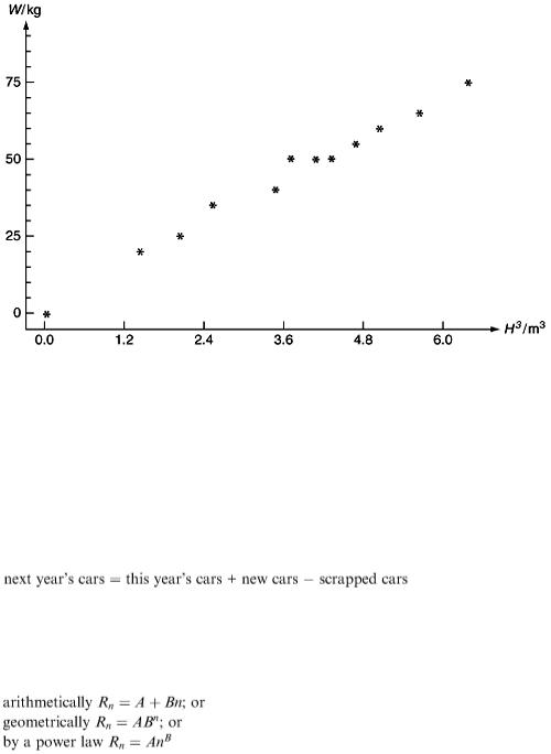
Figure 8.7
Example 8.5
How many cars will there be on the roads of the UK by the year 2020?
Table 8.3 gives data on private vehicles from 1981 to 1997. The variables of interest can conveniently be modelled as discrete variables C n and R n where n represents the number of years since 1981 and C and R stand for cars and new registrations respectively measured in thousands.
Every year new cars are added to the existing stock but also some older cars are scrapped, so a simple model is:
which we can translate into symbols as C n +1 = C n + R n − S n . Let us assume that a constant percentage of currently licensed cars are scrapped every year. This is equivalent to saying that S n = α Cn for some constant α. From the table we note that the number of new cars registered increased every year except for 1990, 1991 and 1993. We could model this increase in three simple ways:
What are the arguments for or against these various options?
The arithmetic model is easy to fit to data but (with B > 0) implies that the number of new cars goes on rising into the future, forever. The geometric model
Table 8.3
with B > 1 also gives an ever-increasing graph, in fact it gets steeper with increasing n. The power model can give an increasing graph which gradually becomes less steep if we take B < 1. To help us make the choice let us plot R n against n as in Figure 8.8.
There is no strong evidence for or against any of the options, so we will use the simple arithmetic form first. Using the least-squares method we find the best fit is R n = 1639 + 21.35 n. We can also test our assumption about scrapped cars since, from the model, S n = C n + R n − C n +1 . The plot of S n against C n is shown in Figure 8.9 and suggests that we might as well take S n to be constant around 1400.
Our model now becomes C n +1 = C n + 239 + 21.35 n. Figure 8.10 compares the model with the data and suggests that it could be used with reasonable confidence to make predictions for a few years ahead.
To get a prediction for the year 2020 we have to continue right up to n = 39 where we find C 39  40 657. We should be worried, however, about extrapolating a model so far beyond the range of our data, especially when we remember the assumptions of an ever-increasing production of new cars and the constant 1400 per year scrap rate. Perhaps the power model with B < 1 would be a safer option? We can fit this model by taking logs, log R n = log A +Blog n. Using the least-squares method on the data values for log R n = 7.325 + 0.091 log n. This gives R n = exp (7.325) × n 0.091 and the resulting model for C n is C n +1 = C n + 1518 n 0.091 − 1400. Figures 8.11 and 8.12 give a comparison of the two models we have used.
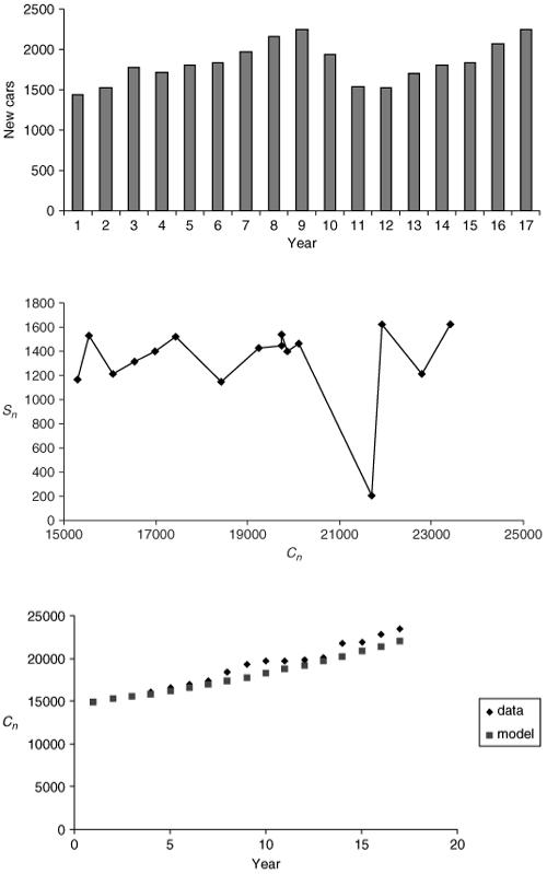
Figure 8.8
Figure 8.9
Figure 8.10
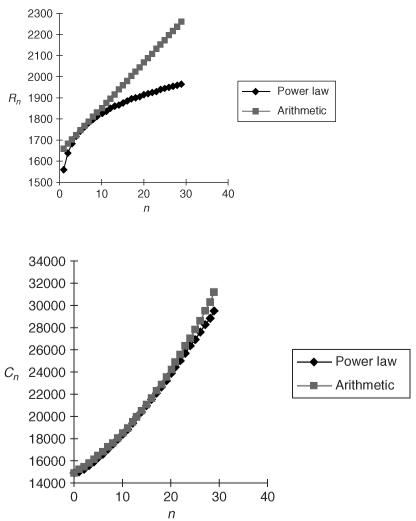
Figure 8.11
Figure 8.12
Example 8.6
In agriculture it can be useful to predict how quickly an animal is likely to grow. One of the factors affecting growth is obviously the rate of feeding. If G denotes the growth rate as measured by the daily gain in weight of an animal (kg d −1 ) and F is the rate of feeding (kg d −1 ), what is the relationship between F and G ? Obviously there is a minimum value of F, F min , below which the animal will loose weight instead of gaining. The smallest possible value of F is 0 in which case the animal will gradually starve to death. We can write these ideas down mathematically as G ≤ 0 when F ≤ F min and G = G s (a negative number) when F = 0. At large feeding
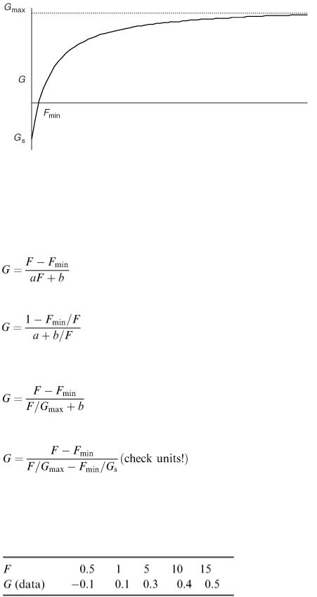
Figure 8.13
rates G is obviously going to be larger but there must be some limit G max . The relationship between F and G can therefore be represented by a model such as the one illustrated in Figure 8.13.
What kind of mathematical model can we use? Since G = 0 when F = F min we can have something like ( F − F min ) in the model. The behaviour for large F can be modelled by a factor of the form 1/ ( aF + b ), so a possible model is:
This is 0 when F = F min and what happens at large F can be seen by writing it as
When F is large F min / F and b/F are both small so this gives G = 1/ a which we want to equal G max , so a = 1/ G max and we have:
When F = 0 this is − F min / b which we want to equal G s so b = − F min / G s and the model is:
This has three parameters, F min , G s and G max . These all represent physically meaningful concepts but measuring them directly would be rather difficult in practice. In theory we could measure G s by starving the animal. We could find F min by trial and error and G max by force-feeding. It would be rather more humane to use data to find estimates of these parameters; suppose the following data is available.
In EXCEL we enter the data and type in the model G (model) = ( F − F min )/( F / G max − F min / G s ). Using the SOLVER tool we minimise Σ( G (model) − G (data)) 2 , allowing the cells containing G
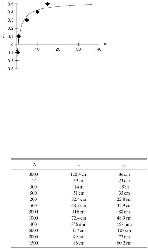
max , F min and G s to change. This leads to F min = 0.764, G max = 0.519 and G s = −0.296. The final model is G = ( F − 0.764)/(1.927 F + 2.581) and the fit to the data is shown in Figure 8.14.
Figure 8.14
An alternative model which also has the right kind of behaviour is G = G max (1 − e − kF ) except that this gives G (0) = 0 instead of G s . We could modify the model to G = A (1 − e − kF ) + G s for some constant A to take care of the condition at F = 0. For large F this gives A + G s so we want A = G max − G s and the model is G = ( G max − G s )(1 − e − kF ) + G s . A fit to the data can be made in the same way as before, using the EXCEL SOLVER to find values of G max , G s and k. What is k in terms of the other parameters G max , G s and F min ? Does this model give a better or worse fit than the other model?
Exercises
The following table gives for each of a sample of jigsaw puzzles, the number of pieces ( N ) and the dimensions ( x and y ) of the finished puzzle. Making a reasonable assumption, formulate a model relating N, x and y.
8.11
Plot the data and fit your model. Given that another puzzle measures 60 cm by 46 cm use your model to estimate the number of pieces. If another puzzle has 300 pieces what size would you