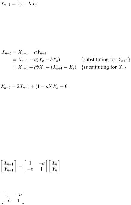
Here we have two explicit but coupled difference equations, neither one can be solved on its own. However, given initial sizes X 0 and Y 0 for the two armies, and also given the parameters a and b, we could compute X 1 and Y 1 etc. directly from the above difference equations, probably on a spreadsheet.

An alternative approach is to eliminate one of the variables by substitution. The first equation implies that

This is

a second -order difference equation. From it we can generate a sequence of X n values provided two starting values, e.g. X 0 and X 1 , are available. Alternatively a mathematical solution for X n in terms of n can be derived. Methods for doing this can be found in the Bibliography.

Both models are considered again in chapters 6 and 9.

5.5 Matrix models

Linear difference equations involving more than one variable can be neatly expressed using vectors and matrices. We have already used this approach on p. 38, chapter 2. The state of the battle in the previous example can be represented by the vector Z n = [ X n , Y n ] and the pair of simultaneous difference equations can be written

so the progress of the battle from one step to the next can be written concisely as Z n +1 = MZ n where M is the matrix

and the solution can be written Z n = M n Z 0 . This approach is especially useful for models representing transitions between states or compartments. When developing models for populations, for example, we often want to do more than just predict the total size of the population. At any time a human population will consist of a mixture of individuals of different age, sex, occupation etc. In order to make forward planning for the provision of resources such as schools and hospitals we need to make predictions about the future numbers of individuals in different categories within the population. We have introduced this in the fish harvest model, Example 2.7.

Example 5.7

Let us take a simple and artificial example of a population of animals, which become adult and capable of reproducing at the age of one year. Suppose we represent the population at time step n in terms of

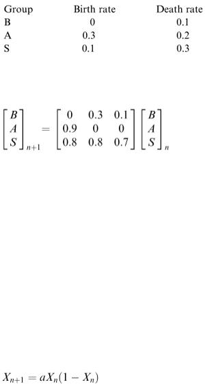
the numbers of animals in each of three categories.

B n = number of babies and young animals up to one year old A n = number of young adults up to two years old, and

S n = number of ‘senior’ adults aged two or older

There will be different annual birth and death rates for the three groups. Suppose we have the following information:

This means, for example, that 90% of babies survive to become adults and that 10% of senior adults produce one offspring per year on average. When we go from year n to year n + 1 we can put this information into matrix form as:

This is a difference equation of the form X n +1 = AX n i.e. like we had in section 5.1 except that now each X n is not a single number but a vector of three numbers and A is not a single number but a matrix.

To find out what happens to the population we only have to keep multiplying by the matrix (often called the transition matrix ). The nature of the solution, and whether we eventually reach a steady state depends on the largest eigenvalue, λ, of this matrix.

If λ > 1 then the population grows without limit.

If λ = 1 then the population converges to the eigenvector associated with λ. If λ < 1 then the population continually decreases.

(See the Bibliography for further information.)

5.6 Non-linear models and chaos

A simple (and important) example of a non-linear difference equation is:

where a is a constant and 0 < X 0 < 1. The solutions of non-linear equations reveal a much stranger and more varied behaviour than that of linear equations and in some cases show the kind of behaviour described as ‘chaos’. This is what happens with the above equation for certain values of a. We can describe the behaviour as follows.

For 0 < a < 1, X n continues to decrease towards zero as in Figure 5.6.

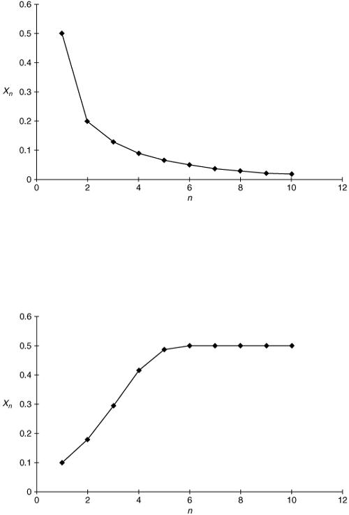
Figure 5.6

For 1 < a < 3, X n increases or decreases (depending on X 0 ) towards the limit 1 – 1/ a as in Figure 5.7.

For 3 < a < 3.449, after a while X n latches on to two distinct values and continues to switch between them for ever. It behaves like a sequence with period 2 as in Figure 5.8.

For 3.449 < a < 3.544, after a while X n jumps between four distinct values, i.e. it has period 4 as in Figure 5.9 and for 3.544 < a < 3.564 we get period 8.

Figure 5.7

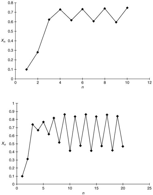
Figure 5.8

Figure 5.9

This ‘period doubling’ continues as we continue to increase a until a approaches the special value 3.57

– when X n jumps between an infinite number of distinct values giving the appearance of a random sequence. This is chaos. It is a fairly recent discovery and has possible applications in a wide variety of areas (see the Bibliography for further information). An effect which has become known as the ‘butterfly effect’ is that a tiny alteration in