


156 Combining Queries for Efficiency
You can see how this feature allows users to enrich and transform data coming from different sources, without the need to make any change to the data source directly.
Joining methods
In the previous recipe, you had the chance to see how to perform a merge where you reference a main table enriched with data coming from another table with geographical details. In fact, there are many ways to join data on matching values following a logic that belongs to traditional relational databases—for example, left/right/full outer joins, inner joins, and left/right anti-joins. These different methods allow users to match data by applying custom logic.
In this recipe, you will see how you can effectively leverage some of the most popular joining methods.
Getting ready
For this recipe, you need to download the following files:
•FactInternetSales CSV file
•DimTerritory2 CSV file
In this example, we will refer to the C:\Data folder.
How to do it…
Once you open your Power BI Desktop application, you are ready to perform the following steps:
1.Click on Get Data and select the Text/CSV connector.
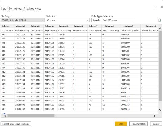
2.Browse to your local folder where you downloaded the FactInternetSales CSV file and open it. The following window with a preview of the data will pop up; click on Transform Data:
Joining methods 157
Figure 5.9 – CSV data preview
158Combining Queries for Efficiency
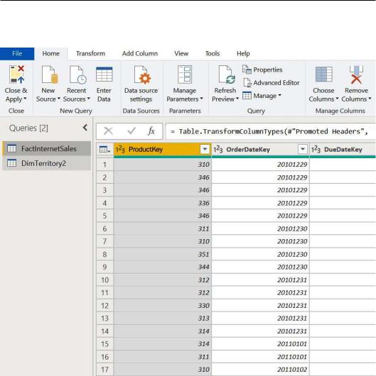
3.Repeat Steps 1 and 2 for the DimTerritory2 CSV file in order to end up with the following two queries in the Power Query UI:
Figure 5.10 – Power Query UI
4.In this case, we want to enrich DimTerritory2 with aggregated data coming from the FactInternetSales table by performing a right outer join. For this, you need to select DimTerritory2 in the Queries pane, browse to the end of the
Home tab, and click on Merge Queries:
Joining methods 159
Figure 5.11 – Merge Queries button
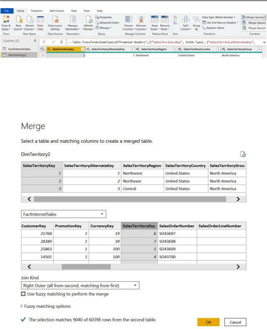
5.Select SalesTerritoryKey from the DimTerritory2 query and
FactInternetSales from the drop-down menu, selecting the same matching value. In the Join Kind field, select Right Outer (all from second, matching from first) and click on OK:
Figure 5.12 – Merge window
160Combining Queries for Efficiency
6.In the DimTerritory2 query, you can find a subset of three rows we had in the original table (DimTerritory) from the previous recipe and a row with null values. When merging with a right outer join, you enriched the DimTerritory2 table with both matching and non-matching values. Click on the Expand icon
on the left of the FactInternetSales column, flag Aggregate, select Sum of TotalProductCost and Sum of SalesAmount, unflag Use original column name as prefix, and click on OK:
Figure 5.13 – Expanding merged column
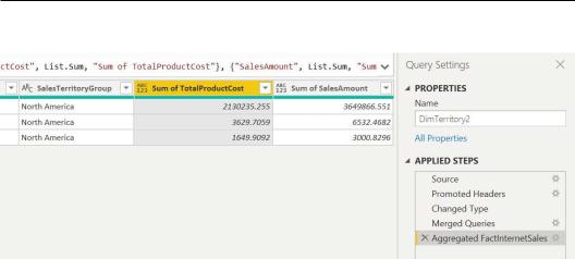
7.You can see two new columns containing data from the FactInternetSales table:
Figure 5.14 – Added columns
Joining methods 161
You can see that in this way, you can add aggregated data and enrich tables with external data. This is useful when you need both matching and non-matching data. In this recipe, you added aggregated sales and total cost values for the geographies available in the DimTerritory2 table, and you also added a row that does not have a match to represent sales and total costs for geographies that are not mapped.
In the previous recipe, you saw how to enrich data coming from other queries. In some cases, you may need to enrich data only on matching values, as you will see in the following exercise.
If you double-click on the Merged Queries step on the APPLIED STEPS pane, you can change and explore other join possibilities. Follow the next steps to see how:
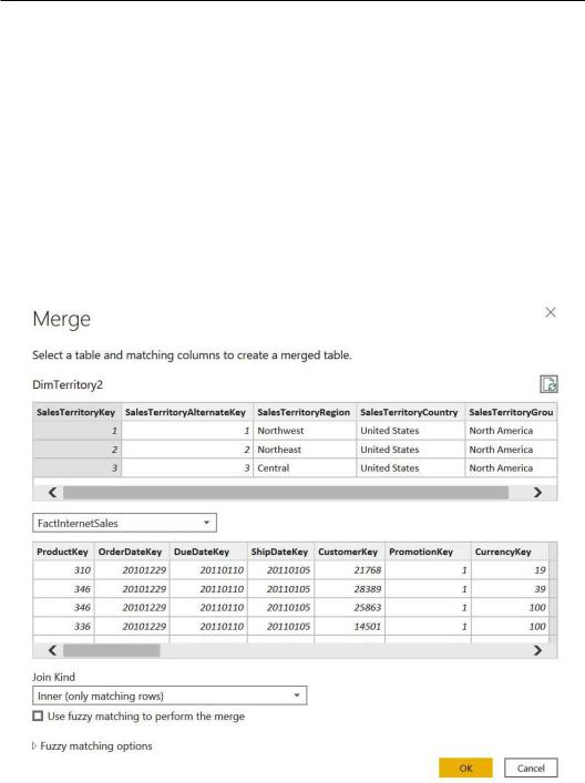
1.Edit the Merge Queries step by double-clicking on it, wait for the Merge window to appear, change Join Kind to Inner (only matching rows), and click on OK:
Figure 5.15 – Merge window
162Combining Queries for Efficiency
2.You can see that in this way, we only added matching information:
Figure 5.16 – Inner join output
Let's add another query to test another join method, Left Anti:
1.Click on Get Data and select the Text/CSV connector.
2.Browse to your local folder where you downloaded the DimProduct CSV file and open it. A preview of the data will pop up; click on Transform Data.
3.Select DimProduct from the Queries pane, browse to the Home tab, and click on
Merge queries.
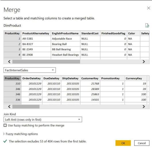
4.Select ProductKey from the DimProduct query and FactInternetSales from the drop-down menu, selecting the same matching value. In the Join Kind field, select Left Anti (rows only in first) and click on OK:
Joining methods 163
Figure 5.17 – Merge window
The idea with this join kind is to have a dataset with all rows from the first table less the matching rows from the second table. If the DimProduct table originally has 404 rows, after this join it will have 53 fewer rows, which are the rows that are matching from FactInternetSales.
164Combining Queries for Efficiency
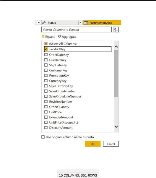
5.Click on the Expand icon on the left of the FactInternetSales column, flag Expand, select ProductKey, and click on OK:
Figure 5.18 – Expanding merged column
6. You can see that the number of rows is reduced in the bottom left of the page:
Figure 5.19 – Updated number of rows
As we observed in this recipe, there are many ways to perform merge transformations, and each allows us to get different outputs of data. You can enrich data, reduce it, retrieve values for each row, or perform built-in aggregations. This step allows you to easily edit update join transformations and tells you which data to expand.