

28 |
POWER EXCEL WITH MR EXCEL |
|
|
I have no idea how Excel knows how to do this. Apparently, Microsoft programmed in a bit of logic to re- member the first column you tabbed out of. When you switch from Tab to Enter, Excel will jump down one row and back to that column. Amazing. If you make a mistake in a previous cell, use Shift+Tab to move backwards through the list.
ENTER DATA IN A CIRCLE (OR ANY PATTERN)
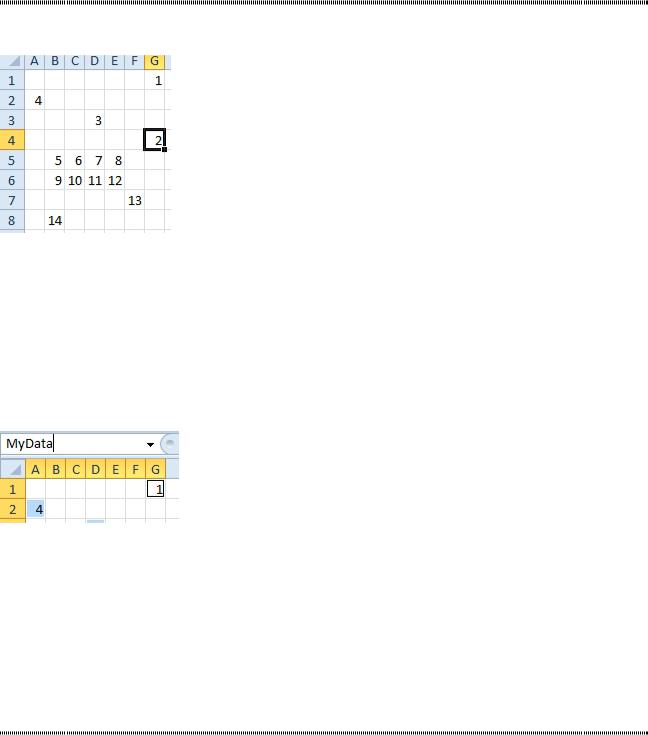
Problem: I need to fill out a form in which the data fields jump all over the place. I start in cell H1, then jump to H5, then E4, then B2, and so on. This figure shows the sequence of fields I have to fill out.
Figure 60 You want to enter data in this sequence.
Strategy: You can use the method described in “Return to the First Column After Typing the Last Col- umn” to solve this problem. The solution relies on the fact that Excel can remember the sequence in which you select cells. Follow these steps:
1. For now, ignore cell 1. Click in cell 2. 2. Hold down the Ctrl key and click cell 3.
3. Keep holding down the Ctrl key while you select cell 4, 5, 6, and so on, in order. (Yes, it absolutely matters that you select the cells in the correct order.)
4. After you select the last cell, keep holding down the Ctrl key and select cell 1.
5. Click the mouse in the Name box (the area to the left of the formula bar that shows an address like H1) and type MyData. Press Enter. Nothing will happen. The Name box will return to saying H1.
Figure 61 Name the selected range.
6. Save the file.
When you need to fill in the cells, select the Name box dropdown and choose MyData. Cell 1 will be se- lected. Type a value and press Enter. Excel will jump to cell 2. Keep typing values and pressing Enter, and
Excel will jump to the fields in the correct order.
Additional Details: This technique works because Excel defines the named range as a specific sequence of cells.UseFormulas,NameManager,Edit.Youwillseethatthenameisdefinedinthesamesequenceasyou selected the cells: “=Sheet1!$G$4,Sheet1!$D$3,Sheet1!$A$2,Sheet1!$B$5,Sheet1!$C$5,Sheet1!$D$5,Shee t1!$E$5,Sheet1!$B$6,Sheet1!$C$6,Sheet1!$D$6,Sheet1!$E$6,Sheet1!$F$7,Sheet1!$B$8,Sheet1!$G$1”.
HOW TO SEE HEADINGS AS YOU SCROLL AROUND A REPORT
Problem: I have a spreadsheet that has headings at the top. I want to scroll through the data and always see the headings.
PART 1: THE EXCEL ENVIRONMENT |
29 |
|
|
Figure 62 You want to see row 3 headings even if you scroll to row 800.
Strategy: Select one cell in the data. Press Ctrl+T and click OK. Your data will be formatted. When you scroll the headings out of view, the headings will replace column letters A, B, C.
1
Figure 63 Tables will keep the headings in view.
This strategy uses the table concept introduced in Excel 2007. It automatically adds Filter dropdowns and formats the table. It also precludes the use of some features like the View Manager. For a more flexible strategy, use Freeze Panes as discussed next.
Alternate Strategy: You can use the Freeze Panes command on the View tab. In order to make the Freeze
Panes command work, you must place the cell pointer in the correct location before using the command.
In the spreadsheet shown in Figure 62 it would be really handy to have row 3 always visible while you scroll. Here’s how you make that happen:
1. Use the arrow at the bottom of the vertical scrollbar to move row 3 to the top of the window.
2. Place the cell pointer in cell A4. You’re going to use the Freeze Panes command, which will freeze all visible rows above the cell pointer and all visible columns to the left of the cell pointer. If you place the cell pointer on the heading for column A, you will not freeze any columns, only the rows.
Figure 64 Cells above and left of the active cell is frozen.
3. With the cell pointer in cell A4, select View , Freeze Panes , Freeze Panes. A solid horizontal line will be drawn between rows 3 and 4. As you scroll down, you will always be able to see the heading rows.
Additional Details: To turn off this feature, go to the View tab and select Freeze Panes, Unfreeze Panes. The Unfreeze Panes menu item is visible only after you have frozen the panes.
See Also: “How to See Both Headings and Row Labels as You Scroll Around a Report,” “How to Print Titles at the Top of Each Page”
30 |
POWER EXCEL WITH MR EXCEL |
|
|
HOW TO SEE HEADINGS AND ROW LABELS AS YOU SCROLL AROUND A REPORT
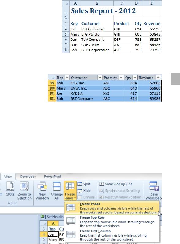
Problem: I have a wide spreadsheet. There are headings at the top of the spreadsheet, and there are sev- eral columns of labels at the left side of the spreadsheet. I also have monthly sales figures that extend far to the right. I need to be able to scroll through the sales figures while always seeing both the headings at the top and the labels at the left of the spreadsheet.
Figure 65 See columns A:F as you scroll right.
Strategy: Use the Freeze Panes command on the View tab. You must place the cell pointer in the correct location before using the command.
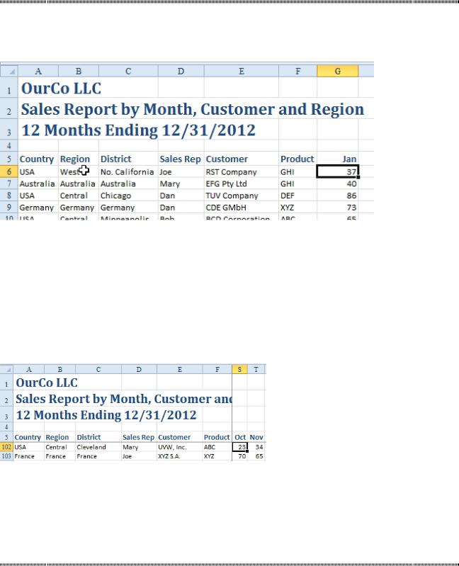
In the spreadsheet shown above, you might want A1:F5 visible all the time. Then, you could scroll through the monthly figures and always be able to see the customer information in the left columns and the month name information in row 5. Here’s how you make it happen:
1. Select cell G6. This is the first non-frozen cell.
2. Select View, Freeze Panes, Freeze Panes. You will see a solid line between columns F and G and between rows 5 and 6.
Results: As you scroll, you can always see the headings.
Figure 66 Scroll out to October and you can still see A:F.
Alternate Strategy: Some people prefer to use Split instead of Freeze Panes. I am not a fan of Split since it is too easy to scroll from one quadrant to another. However, several viewers provided reasons why they prefer Split. Search YouTube for “Learn Excel 1101” for a demo on using split.
Note that the Split handles were removed after Excel 2010.
WHY IS THE SCROLLBAR SLIDER SUDDENLY TINY?
Problem: I have a worksheet with two or three screens of data. I can easily grab the vertical scrollbar and move to the top or bottom of the data set. Something happened, and now the huge scrollbar slider has become really tiny. Further, if I move it just one pixel, instead of jumping to the next screen of data, Excel will move to row 4500.
PART 1: THE EXCEL ENVIRONMENT |
31 |
|
|
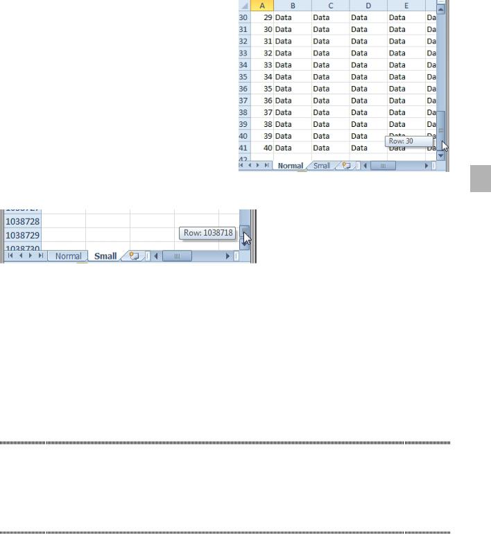
Figure 67 Normally, the slider will take you to the last row with data. |
1 |
Strategy: Someone pressed End+Down Arrow key to move to row 1048576.
Figure 68 Accidentally activate a cell at the bottom. The slider is tiny.
You can often restore the size of the slider by moving it completely to the top of the spreadsheet. If this does not work, then there is one rogue cell way below your data that has become activated. Perhaps some- one pressed the Spacebar or applied text formatting or something. Follow these steps:
1. Note the last row that you believe to contain data.
2. Press the End key and then press the Home key. Excel will jump to the intersection of the last active row and the last active column. This row is usually way beyond the row that you believe to be the last row.
3. Delete all rows from the bottom of your data set to the rogue last row. 4. Save the workbook. The scrollbar slider will return to full size.
Saving the workbook is the key. Even after you delete the extra rows, Excel will not restore the size of the scrollbar.
WHY WON’T MY SCROLLBAR SCROLL TO MY CHARTS?
Problem: I have 100 rows of data and then 50 rows of charts. When I drag the scrollbar to the bottom, it only shows my data, not the charts.
Strategy: This is fixed in Office 365, but if it is still happening to you, go to a row below the charts, type a few spaces. That row will now become active and the scroll bar should adjust.
JUMP TO THE EDGE OF THE DATA
Problem: I have thousands of rows of data. I want to quickly move to the edge of the data using my mouse. Strategy: To jump to the bottom of the data, double-click the bottom edge of the active cell.