

110 |
|
POWER EXCEL WITH MR EXCEL |
|
||
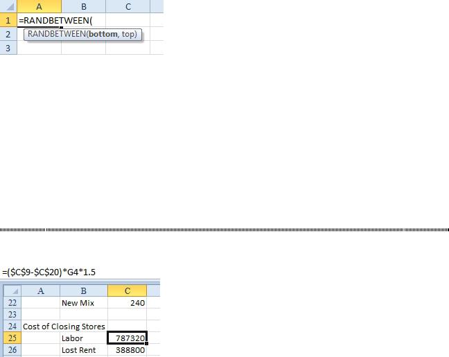
Here is how you’re supposed to use AutoComplete: |
||
1. |
Type =RA. Excel displays a list of five functions. |
|
2. |
Use the down arrow to move to RANDBETWEEN. Excel will show a ToolTip to indicate that the |
|
3. |
function will return a random number between the numbers you specify. |
|
Press the Tab key to accept the function and move to the arguments. I was used to using the Tab key |
||
|
here because I’ve been using AutoComplete in VBA for a while. However, many people try to press |
|
|
Enter here, which leads to a #NAME? error. After you press the Tab key, Excel fills in the function |
|
|
name and the opening parenthesis. |
|
Figure 269 Press Tab to finish typing the selected function name.
Gotcha: I will sound ungrateful, but Microsoft types the opening parenthesis for you. I cannot seem to break the habit of typing the opening parenthesis myself. Going back to the days of typing @SUM(, or even typing =SUM(, my fingers automatically type the opening parenthesis. I cannot type =RANDBETWEEN( without typing an opening parenthesis. Here, let me try a few more: =VLOOKUP( =AVERAGE( =TRIM( =MID( =ROMAN(. My brain is simply hard-wired to type that opening parenthesis. I don’t even conscious- ly think about typing the parenthesis. It simply just gets typed.
So, as you can guess, every time I use AutoComplete, I get an error saying that I’ve typed too many pa- rentheses.
I don’t have a good solution for this, other than trying to retrain yourself not to type the opening parenthesis.
USE F9 IN THE FORMULA BAR TO TEST A FORMULA
Problem: I have a complex formula that does not appear to be providing the correct result. The formula has multiple terms, and I am not sure which part is not working correctly.
Figure 270 Troubleshoot this formula.
Strategy: You can use F9 to test a formula. Here’s how:
1. Select cell C25 and press F2 to put the cell in Edit mode. In this mode, each cell reference in the for- mula is color coded. The $C$9 text in the formula is blue, and the outline around C9 is blue.
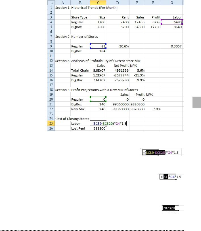
PART 2: CALCULATING WITH EXCEL |
111 |
|
|
2
Figure 271 In Edit mode, the formula references are color coded.
2. To selectively calculate just a portion of the formula, use the mouse to highlight a portion of the formula.
Figure 272 Select part of the formula.
3. Press the F9 key. The highlighted portion of the formula will be replaced with the current result of the formula.
Figure 273 Press F9 to calculate the highlighted portion.
4. Press the Esc key to return to the original formula.
Additional Details: If you press F9 without selecting anything, it will calculate the entire formula and replace it in the result.
Figure 274 Press F9 to calculate the entire formula.
QUICK CALCULATOR
Problem: I need to find a quick answer to a mathematical problem, and I don’t have a calculator. Can
Excel help?
Strategy: You can use Excel as a simple calculator. Follow these steps:
1. Go to a blank cell.
2. Type an equals sign.
3. Enter a calculation.
112 |
POWER EXCEL WITH MR EXCEL |
|
|
Figure 275 Type = and a calculation in a blank cell.
4. Press the F9 key. Excel will display the result.
Figure 276 The result..
5. Press the Esc key to clear the cell.
You can start a formula with equals, plus, or minus signs. You could also have typed +14215469*5.
WHEN ENTERING A FORMULA, YOU GET THE FORMULA INSTEAD OF THE RESULT
Problem: When entering a formula, Excel shows me the formula in the cell instead of the result.
Figure 277 Excel displays the formula.
Strategy: There are three possible problems in this case.
Possibility 1: You may have forgotten to start the formula with an equals sign.
Figure 278 You forgot to start the formula with an equals sign.
Follow these steps to correct the formula:
1. Select the cell and press F2 to edit the cell.
2. Press the Home key to go to the beginning of the formula.
3. If there see a hidden apostrophe, delete it using the Delete key. 4. Type the = sign.
5. Press Enter. Excel shows the result.
Possibility 2: The cell might have been assigned the numeric format @, which is the code for a text cell.
The maddening part of this problem is that this format can get set even without you knowing it. A column can inherit a text format if you import a text file and use the text setting for the import. Here’s how you fix this problem:
1. Select the problematic cell. Look in the Number group in the Home tab of the ribbon. 2. Confirm that the cell has a Text format assigned.
Figure 279 Text formats will show the formula and not the results.
3. Change the cell to any format other than Text.
4. This does not fix the formula! Edit the cell using the F2 key and then press Enter.
Possibility 3: The third possibility, which is the least likely, is that you are in Show Formulas mode, as shown here. In this mode, all the cells that have formulas show their formulas.
PART 2: CALCULATING WITH EXCEL |
113 |
|
|
Figure 280 See all formulas.
To fix this problem, you press Ctrl+` to toggle in and out of Show Formulas mode. (On U.S. keyboards, this character is below the Esc key, on the same key as the tilde.)
When a cell shows a formula rather than a result, there are three possible reasons: (1) You forgot to start the formula with an equals (=) sign, (2) the cell is not formatted for numeric data, or (3) the worksheet is in Show Formula mode.
HIGHLIGHT ALL FORMULA CELLS USING CONDITIONAL FORMATTING
Problem: I need to audit a worksheet created by a former co-worker. How can I mark all formula cells?
Strategy: There are two great ways to do this. The first is a one-time snapshot of current formulas. The 2 second will continually update so you can see if someone types a plug number where a formula should be.
To do a one-time snapshot go to Home, Find & Select, Formulas. Go to the Font color or Fill color and apply a color. All of the formula cells will be highlighted.
To have the formulas be highlighted using conditional formatting, follow these steps:
1. Select the used range of your worksheet. Note the top left cell (usually A1, but it might be something else).
2. Home, Conditional Formatting, New Rule, Use a Formula. Type this formula: =ISFORMULA(A1).
Adjust the A1 if the top left cell of your selection is not A1. 3. Click Format and apply a fill color. Click OK.
All formulas will be highlighted. If a formula gets replaced by a constant, the fill color will disappear.
YOU CHANGE A CELL IN EXCEL BUT THE FORMULAS DO NOT CALCULATE
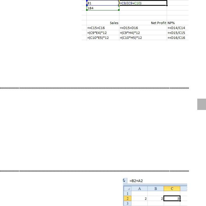
Problem: Sometimes when I change a cell in Excel, the formulas do not calculate. Below, cell C2 indicates that two plus two is not four.
Figure 281 Excel isn’t calculating.
Strategy: In this case, someone has put the worksheet in Manual calculation mode. You can try pressing
F9 to calculate.
There are several variants of recalculating:
●● Pressing F9 will recalculate all cells that have changed since the last calculation, plus all formulas that depend on those cells in all open workbooks.
●● For quicker calculation, use Shift+F9. This will limit the calculation to the current worksheet.
●● For thorough calculation, use Ctrl+Alt+F9. This will calculate all formulas in all open workbooks, whether Excel thinks they have changed or not.
●● Pressing Ctrl+Shift+Alt+F9 rebuilds the list of dependent formulas and then does a thorough cal- culation.