Figure 334 Round .5 towards the even number.

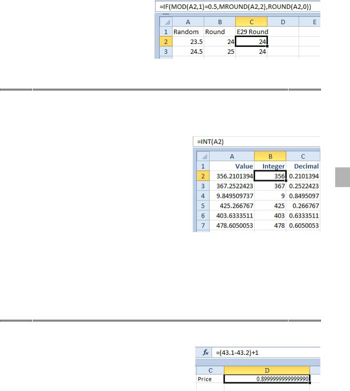
SEPARATE THE INTEGER FROM THE DECIMALS

Problem: I have a column of values that include digits before and after the decimal point. I don’t want to round anything, I just want the whole number. Or, I just want the decimal. How can I easily break those apart?

Strategy: Use the INT function to return the integer portion of the number.

2

Figure 335 Use INT to chop the decimals off your numbers.

To lose the integer and keep only the decimals, I use =A2-INT(A2). Another solution is to use MOD(A2,1).

The MOD function is equivalent to the math concept of modulo. Divide A2 by 1 and return the remainder.

Gotcha: the INT function for negative numbers may not act like you expect. The INT of -9.1 is -10, since this is the integer just less than -9.1. If your values might contain negative numbers, then consider using the TRUNC function to truncate the decimals. For positive numbers, INT and TRUNC are identical. The only difference is for negative numbers. TRUNC(-9.1) will be -9.

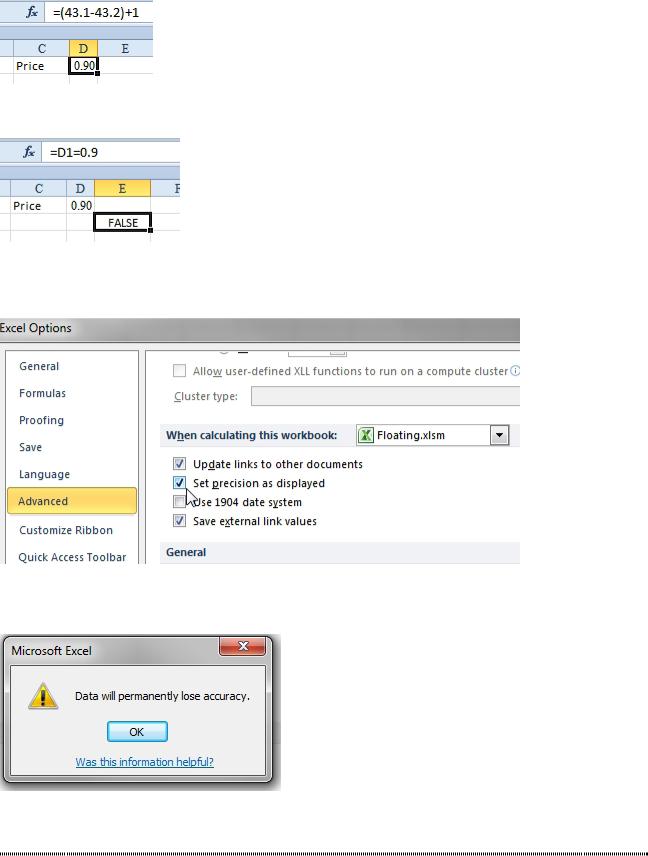
WHY IS THIS PRICE SHOWING $27.85000001 CENTS?

Problem: I have a worksheet in which I expect the cells to show dollars and cents. For some reason, a price in the formula bar is showing a few millionths of a cent.

Figure 336 Not quite 0.90.

Strategy: These stray values can happen due to something called floating-point arithmetic. Whereas you think in 10s, computers actually calculate with 2s, 4s, 8s, and 16s. Excel has to convert your prices to 16s, do the math, and then present it to you in tenths. A simple number like 0.1 in a base-10 system is actually a repeating number in binary.

Sometimes seemingly bizarre rounding errors creep in. There is one quick solution, but you have to be careful when using it:

1. Format your prices to have two decimal places. Use either the Format Cells dialog or the Decrease

Decimal icon.

Figure 337 Still not 0.90.

Things now look OK, but if you ever test to see if this value is really 0.90, it will return FALSE.

Figure 338 The formatting is showing 0.90, but the cell really isn’t 0.90.

2. Select File, Options, Advanced. In the Calculation Settings For This Workbook section, select Set Precision as Displayed. Using this setting, Excel will truncate all values to only the number of deci- mal places shown.

Figure 339 Eliminate the tiny floating point errors.

Gotcha: There is neither an Undo command nor any other way to regain those last numbers. However,

Excel will warn you that your data will permanently lose accuracy.

Figure 340 This warning displays while in the Options dialog.

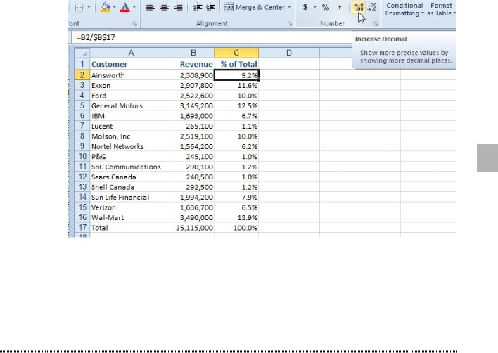
CALCULATE A PERCENTAGE OF TOTAL

Problem: I have a spreadsheet with sales by customer and a total at the bottom. I want to express each customer as a percentage of the total.

Strategy: Divide each row’s sales by the total cell. Follow these steps: 1. Select a cell next to the first revenue cell.

2. Type an equals sign. Press the Left Arrow key.

3.Type the forward slash (/) sign. Press the Left Arrow key. Press Ctrl+Down Arrow key. Your cell pointer should now be on the total cell.

4.Press the F4 key. The formula bar should now show B2/$B$17.

5.Press Ctrl+Enter to enter the formula and stay in the current cell. Format the calculation as a per- centage by using the % icon on the Home tab.

6.To use the format 9.2% (that is, one decimal place) instead of 9%, choose the Increase Decimal icon.

7.In cell C2, double-click the fill handle to copy the formula down to the other rows.

8.Add the heading % of Total in cell C1.

2

Figure 341 Show a percentage of total.

Additional Details: The key element of this procedure is pressing the F4 key to add dollar signs to the reference for the total row. As you copy the formula from C2 to C16, the formula is always going to compare the revenue in the current row to the total revenue in row 17.

Creating a percentage of total is a common task in Excel. Being able to quickly enter an initial formula that can be copied to all cells is a good technique to have in your skill set.

CALCULATE A RUNNING PERCENTAGE OF TOTAL

Problem: I have a report of revenue by customer, sorted in descending order. Management consultants often argue that it’s important to concentrate the best team on the 20% of the customers who provide 80% of the company’s revenue. How can I calculate a cumulative running percentage of the total so I can deter- mine which 20% of customers to focus on?

Strategy: I hate solutions that require two different formulas, but the intuitive solution to this problem is one of them. You will need one formula for cell C2 and a different formula for cells C3 and below. Here’s what you do:

1. In cell C2, enter the formula =B2/$B$18. Format the result as a percentage with one decimal place. 2. Copy C2 to just the next cell, either by dragging the fill handle down one cell or using Ctrl+C and

then Ctrl+V.

3. Press F2 to edit cell C3.

4. Type a plus sign and touch cell C2. Press Ctrl+Enter.

5. Double-click the fill handle in C3 to copy this formula down to all the other cells. Note that you do not want this formula to be added to your total row. As shown below, the data set was purposely set up with the total row and the data separated by a blank row in order to prevent this formula from copying to the total row.

Figure 342 Add this row’s percentage of the total to the previous row.

Alternate Strategy: If you absolutely want to produce this total with a single formula, you could use the formula =SUM(B2:B$2)/B$18 in C2 and copy it down. This works because the range B2:B$2 is an interest- ing reference: It says to add up everything from the current row to the top row. This formula seems a bit less intuitive. For large data sets, it will take much longer to calculate than the first method. (See Consider Formula Speed for details.)

USE THE ^ SIGN FOR EXPONENTS

Problem: I have a room that is 10 feet x 10 feet x 10 feet. How do I find the volume of the cube?

Strategy: The formula for volume is width x length x height. In this case, it is 10 x 10 x 10, or 103. In Excel, the caret symbol (also known as “the little hat,” or “the symbol when you press Shift 6”) is used to indicate exponents. Here’s how you use it to find the volume of your room:

1. In cell B2, enter 10.

2. In cell B3, enter the formula =B2^3.

The result will be 1,000 cubic feet of volume in the room.

Figure 343 The caret raises a number to a power.

RAISE A NUMBER TO A FRACTION TO FIND THE SQUARE OR THIRD ROOT

Problem: Excel offers a SQRT function to find the square root of a number. What do I do if I need to figure out the third root or the fourth root of a number?

Strategy: You can raise a number to a fraction to find a root. To find the square root of a number, you can raise the number to the 1/2 power. To find the cube root of a number, you can raise the number to the 1/3 power. To find the eighth root of a number, you can raise the number to the 1/8 power.

Let’s look at several examples.