

200 |
POWER EXCEL WITH MR EXCEL |
|
|
|
CALCULATE A FORMULA IN SLOW MOTION |
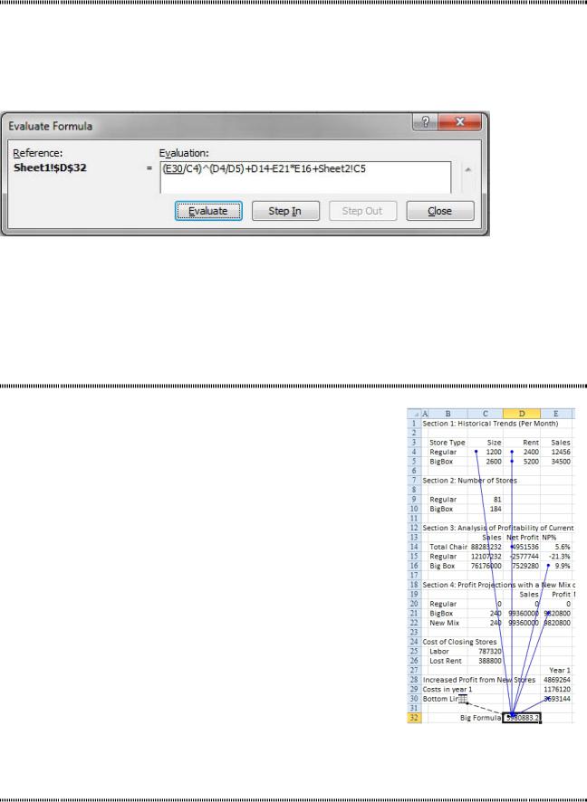
Problem: I am trying to trace how a formula is calculating. What should I do?
Strategy: Use the Evaluate Formula command on the Formulas ribbon tab. You select the cell that con- tains the formula you want to examine. Then you select Formulas, Evaluate Formula.
The Evaluate Formula dialog shows the formula. The first item to be calculated is underlined. Click Evalu- ate to calculate the underlined portion of the formula.
Figure 491 The underlined term will be evaluated next.
With each click of Evaluate, Excel will calculate the underlined portion and show the results in italics. It will underline the next step in the calculation.
Additional Details: Any time the next term to be calculated is a cell reference, you can click the Step In button to evaluate the formula in that cell. You click Step Out to close the most recent detail level and go back one level.
WHICH CELLS FLOW INTO THIS CELL?
Problem: I have a large formula, and I would like to visually see how the cell is calculated.
Strategy: One way to handle this is to select the cell and then press F2 to edit the cell. All the references in the formula will light up with different colors. If the precedent cell is in the visible portion of the window, the cell will be surrounded by a box of the same color as the formula.
Alternate Strategy: If you need a more permanent view of the calculations than pressing F2 provides, you can use the Formula Auditing menu to draw blue arrows from all the precedent cells. To do so, you select cell D32 and then select Formulas, Trace Precedents. Excel will draw blue arrows from all the cells that are referenced in the D32 for- mula. As shown near the bottom left of this figure, the arrow from the other worksheet icon indicates that at least one reference is on another worksheet. Double-click the arrow to see a list of those off-sheet precedents.
If you click Trace Precedents enough times, Excel will trace the precedents of all the arrowed cells. After a few iterations of the command, you will see that nearly all the cells factor in to the calculation.
Figure 492 Trace Precedents.
COLOR ALL PRECEDENTS OR DEPENDENTS
Problem: The auditing arrows are confusing. Can I simply color the precedent or dependent cells?
Strategy: Use Go To Special. Follow these steps. 1. Select one cell in your worksheet.

PART 2: CALCULATING WITH EXCEL |
201 |
|
|
2.Choose Home, Find & Select, Go To Special
3.In Go To Special choose Precedents.
4.You now have a choice. Do you want only the direct precedents or all precedents.
Figure 493 Choose Direct Only or All Levels.
5. Click OK. Excel selects all of the cells that are precedents or dependents.
6. Open the paint bucket menu on the Home tab and choose a color. You now have a permanent indica- tor of the precedents or dependents.
Gotcha: This method will not mark the off-sheet precedents or off-sheet dependents.
MONITOR DISTANT CELLS
2
Problem: I have a massively large spreadsheet. I’m working on calculations in the top of the spreadsheet but need to monitor results in several other worksheets. It is a pain to travel back and forth to monitor those cells. Is there another way to do this?
Strategy: The Watch Window is a favorite tool of VBA programmers, and Microsoft added it to the regular
Excel interface. Here’s how you use it:
1. Select Formulas, Watch Window. The Watch Window, a floating dialog box that you can move around
your screen, will appear.
2. Click Add Watch.
3. Using the Add Watch dialog, navigate to and touch the cell that you want to watch. Alternatively, you can first navigate to the cell, click Add Watch, and click Add.
For each cell that you add to the Add Watch dialog, you can always see the formula and the result of that formula in the Watch Window. You can add cells from other sheets and even from other workbooks.
Figure 494 Watch various cells.
202 |
POWER EXCEL WITH MR EXCEL |
|
|
Additional Details: The cells listed in the Watch
Window act as bookmarks! You can double-click a cell and jump to the cell, even if it is on another worksheet.
Gotcha: If you change the numeric format of a number, it does not automatically appear in the
Watch Window. However, if you double-click the
Value in the Watch Window, it will update.
Additional Details: You can resize the column widths in the Watch Window, as necessary. Further, you can resize the entire Watch Window, and you can even dock it to the top, bottom, or side of the worksheet. Grab the title bar and drag the Watch
Window off the edge of the window. In this figure, the window is docked on the left side of the screen. There is easily room for 3 dozen cells to appear.
Figure 495 Dock the watch window.
AUDITING WORKSHEETS WITH INQUIRE
Problem: I have to compare two versions of a workbook to find what changed.
Strategy: Some editions of Excel ship with the Inquire add-in. This add-in includes the following tools: ●● Analyze workbook for risks, such as hidden cells, hidden sheets, circular references, and more. ●● Map relationships from one workbook to other linked workbooks
●● Map relationships from one worksheet to other worksheets ●● Map which cells are related to the current cell
●● Compare two versions of a workbook
●● Repair the Too Many Cell Formats error
Figure 496 Tools in the Inquire add-in.
Inquire is included in Pro Plus and Enterprise E3 versions of Office 2013 and with the Professional, Pro Plus, and E3 versions of Excel 2016 and Office 365. It is rarely enabled by default. To see if you have In- quire, select File, Options, Add-Ins. From the bottom of the Excel Options dialog, open the Manage dropdown and choose COM Add-ins and click Go.... If Inquire is shown in the list, select it and click OK. The Inquire tab will appear on the right side of the Ribbon.
Figure 497 Inquire is never enabled by default.
PART 2: CALCULATING WITH EXCEL |
|
203 |
|
|
|
|
USE REAL DATES |
|
Problem: I hate Excel dates. I try to do a calculation and I get a number like 43148. Or I try to calculate the number of days between an invoice and a payment and I get an answer like January 15, 1900.
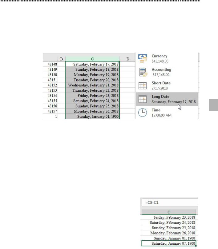
Strategy: It will take five minutes to understand how Excel stores dates. Open a blank worksheet. Type a number in the range of 42000 to 44000 in cell A1. Select that cell. Hold down the Ctrl key while you drag the fill handle down for several cells. At the bottom of the list, enter a 1. Over in column C, enter =A1 and copy it down. You should have two identical columns of numbers.
Select column C. On the Home tab, open the General dropdown and choose Long Date. Column C will change to show dates in the modern era, plus January 1, 1900.
2
Figure 498 Format the numbers as dates.
You haven’t changed the value stored in column C. Cell C1 still contains 43148. You have told Excel to treat the cell as a date and so it calculates a weekday, month, day, and year when applying the formatting.
Additional Details: Excel stores dates as the number of days elapsed since January 1, 1900. Assuming that you are reading this book in the 2017–2021 timeframe, whenever you see a number in the 42700–
44600 range, you might be seeing a date cell that is not formatted as a date.
When I say that you should use “real” dates, I mean to store a number like 43148 in the cell and use nu- meric formatting to display that number as a date. The main advantages of real dates are that you can easily change the format of the date, and you can easily do any calculations that you need with the dates.
You can not do calculations when you have dates that are stored as text.
Gotcha: While Excel is really fast at converting 43148 to a month, day, year, it does a notoriously bad job of deciding whether to format the result of a formula as a number or as a date. Here are two examples:
Go to the bottom of your dates in column C and calcu- late =C8-C1. This formula should calculate the number of elapsed days between the two dates. The correct answer is 7. Excel gets the correct answer, but because that column was previously formatted to show long dates, you will see the 7 converted to Saturday, January 7, 1900.
Figure 499 The correct result of 7 is incorrectly formatted as a date.
To solve the problem, go back to the numeric formatting dropdown on the Home tab and choose Number.
The result will now appear as 7 or 7.00. The problem in this case was that you entered a formula that should return a number in a column that had previously been formatted to show dates.