

PART 2: CALCULATING WITH EXCEL |
183 |
|
|
2
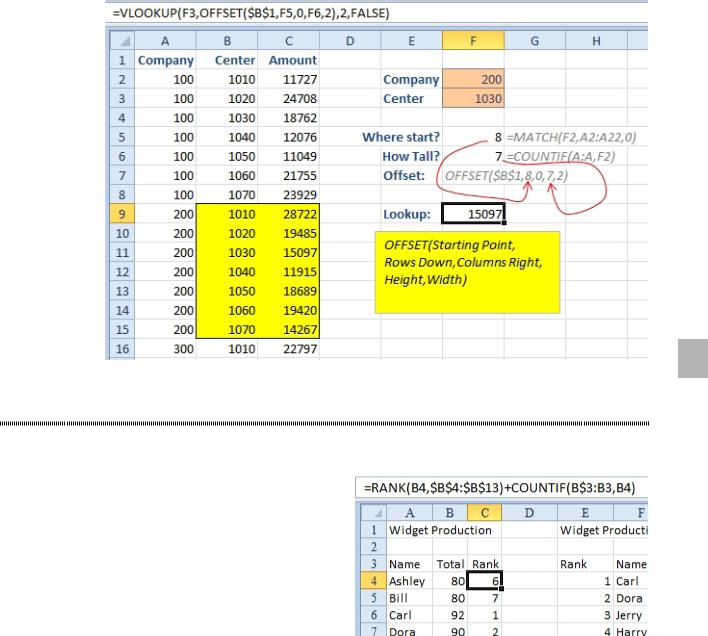
Figure 450 OFFSET is slow, but versatile.
ADD COMMENTS TO A FORMULA
Problem: I spent a great deal of time perfecting the formula shown below. I would like to leave myself notes about it so I can figure it out again six months from now.
Figure 451 Will you remember why you added the COUNTIF?
Strategy: An old Lotus 1-2-3 function—the N function—is still available in Excel. It turns out that N of a number is the number and N of any text is zero. Thus, you can add several N functions to a formula without changing the result, provided that they contain text.
If you have figured out some obscure formula, you can leave yourself notes about it right in the formula.
184 |
POWER EXCEL WITH MR EXCEL |
|
|
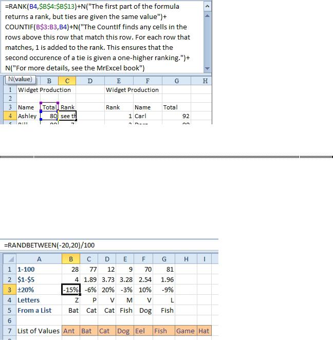
Figure 452 Add your comment as text in the N() function.
CREATE RANDOM NUMBERS
Problem: I want to create a range of random numbers or letters.
Strategy: You use the RANDBETWEEN function. This function will return a random integer between lower and upper limits. Here are some examples:
●● =RANDBETWEEN(1,100) for random integers between 1 and 100.
●● =RANDBETWEEN(100,500)/100 for random prices between $1.00 and $5.00 ●● =RANDBETWEEN(-20,20)/100 for random growth from 80% to 120%/
●● For random capital letters, use: =CHAR(RANDBETWEEN(65,90)).
●● For a random item from a list stored in B7:I7, use =INDEX($B$7:$I$7,RANDBETWEEN(1,8)).
Figure 453 Generate random values.
Additional Details: The last bullet point shows off an interesting and undocumented feature of INDEX.
Normally, you would specify =INDEX(range,row,column). This would mean that you would have to specify =INDEX(B7:I7,1,RANDBETWEEN(1,8)). However, when you range is exactly one row tall, Excel will use the second argument as a column number instead of a row number.
Alternate Strategy: Excel also offers the RAND function, which will return a decimal between 0 and
0.9999999. Instead of using the formula =RANDBETWEEN(1,10), you could use =INT(RAND()*10)+1.
Additional Details: Every time you press F9 or enter a new value in the worksheet, the random numbers will change. You might want to change the formulas to values to freeze the random numbers. To do this, you select the range of random numbers, press Home, Copy, and then select Home, Paste dropdown, Paste
Values to convert formulas to numbers.
Gotcha: These are actually pseudo-random numbers. If you are performing complex modeling involving millions of numbers, patterns may emerge.

PART 2: CALCULATING WITH EXCEL |
|
185 |
|
|
|
|
RANDOMLY SEQUENCE A LIST |
|
Problem: The students in my class must present an oral book report. Rather than have them go alpha- betically, I want to randomly sequence them. How can Excel help me do that?
Strategy: Put the students in column A. Add a =RAND() formula in column B. Sort by column B. Each time that you sort, the students will be in a different sequence.
2
Figure 454 Sort by the RAND() column.
Gotcha: The data is sorted, and then column B is recalculated. It will appear that the new figures in col- umn B are not in any order. This is because the sort was based on the previous values in column B.
PLAY DICE GAMES WITH EXCEL
Problem: My Monopoly set is missing the dice. How can I create a spreadsheet that will simulate ran- domly rolling two dice?
Strategy: You can use the RANDBETWEEN function and clever spreadsheet formatting to simulate two or more dice. Follow these steps:
1. Select cell B2. Select Home, Format, Row Height. Set the row height to 41. 2. In cell B2, enter the formula =RANDBETWEEN(1,6).
3. With cell B2 selected, click the Center and Middle Align buttons on the Home tab of the ribbon.
4. In the Font group of the Home tab, choose the Bold icon. Select 24 point from the font size dropdown.
5. Choose Thick Box Border from the Border dropdown.
6. Copy cell B2 and paste it to cell D2. As shown below, you will have the two dice required for Monopoly.
7. Copy B2 to make additional dice if necessary.
Figure 455 Create dice with Excel.
Results: You will have one die in cell B2 and another in cell D2. Every time you press the F9 key, you will have a new roll of the dice.
186 |
POWER EXCEL WITH MR EXCEL |
|
|
|
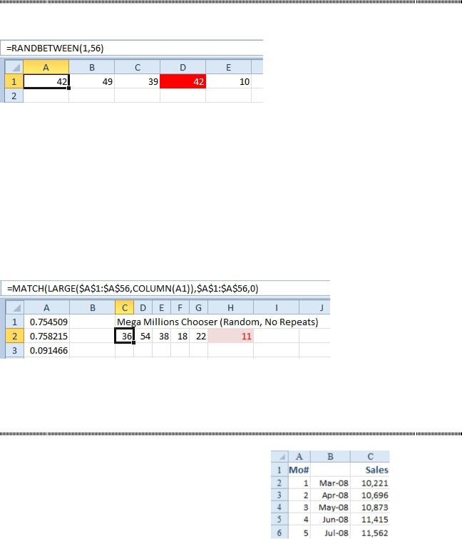
GENERATE RANDOM WITHOUT REPEATS |
Problem: I want Excel to generate numbers for the lottery. Once a number is chosen, I don’t want that number to appear again. Using RANDBETWEEN, it is possible to get duplicates.
Figure 456 Eventually, RANDBETWEEN returns duplicates.
Strategy: to solve this problem, you need to sort the 56 numbers into a sequence and choose the top five numbers from the list. This will prevent any duplicates from showing up.
Say that you want to generate five numbers from 1 to 56. Follow these steps: 1. Select a range that is one column wide by 56 rows tall.
2. Type =RAND(). Press Ctrl+Enter to enter that formula in all of the cells. In my example, I used A1:A56.
From here, you want to find the largest values using =LARGE(A1:A56,1) then =LARGE(A1:A56,2), then LARGE(A1:A56,3), and so on. Once you locate the largest value, use MATCH to find that value within the list. The position in the list represents the lotto number.
3. Combining all of those formulas together, you get =MATCH(LARGE($A$1:$A$56,COLUMN(A1)),$ A$1:$A$56,0). Enter this formula in C2:G2.
4. For the extra ball, use a regular old =RANDBETWEEN(1,46).
Figure 457 You won’t get any repeats in C2:G2.
Additional Details: For PowerBall, enter numbers in A1:A59. Change the 56 in the formula above to a 59. Change the formula in H2 to get numbers from 1 to 39.
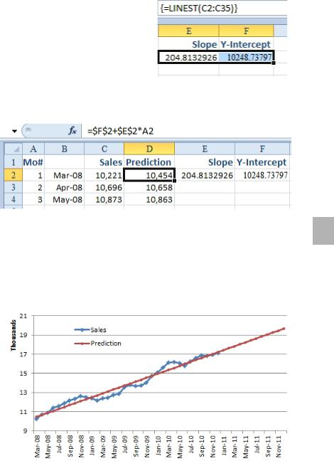
CALCULATE A TRENDLINE FORECAST
Problem: I have monthly historical sales data. I want to predict future sales by month.
Strategy: You can use the least-squares method to fit the sales data to a trendline. Excel offers a function called LIN-
EST that will calculate the formula for the trendline.
Figure 458 Forecast future data.
You might remember from math class that a trendline is represented by this formula: y = mx + b
In this example, y is the revenue for the month, m is the slope of the line, x is the month number, and b is the y-intercept. If you were to look at the data, you might guess that the prediction for a given month is $10,000 + Month number x $400. In this case, the value for b would be 10,000, and the value for m would be 400. This is just my wild guess; Excel can calculate the number exactly.
LINEST is a very special function. Instead of returning one number, it actually returns two (or more) num- bers as the result. If you select a single cell and enter =LINEST(C2:C35), it will return a single number, which is of no help. Entering the formula the wrong way returns a single answer of 204.8133. The first time you do this, you might wonder how the number 204.81 could describe a line.
PART 2: CALCULATING WITH EXCEL |
187 |
|
|
It turns out that Excel really wants to return two numbers from the function. Here’s the trick:
1.Select two cells that are side by side.
2.Type the function in the first cell. After you type the closing parenthesis, press Ctrl+Shift+Enter. Excel returns both the slope and the y-intercept.
Figure 459 The results appear in 2 cells.
3.Add a Prediction column. In column D, enter a formula to calculate the predicted sales trendline. The formula is the intercept in F2 plus the slope in E2 times this row’s month number.
Figure 460 Use the results of the LINEST to predict sales.
You will now be able to graph columns B:D to show how well the prediction matches the historical actuals. |
2 |
|
|
Additional Details: When the data along one axis of your data contains dates, it is best to delete the |
|
heading in the upper-left corner of your data set before creating the chart. You clear cell B1, select B1:D47, |
|
and select Insert, Line, Line with Markers. As shown below, the resulting chart shows that the predicted |
|
trendline comes fairly close to the actuals. You can also see that the formula predicts that you will be sell- |
|
ing almost $20,000 per month one year from now. |
|
Figure 461 Plot actuals vs. forecast to see if the sales match a trend.
Gotcha: When you select two cells for the LINEST function, they must be side by side. If you try to select two cells that are one above the other, you will just get two copies of the slope.
Alternate Strategy: A different method is to use the INDEX function to pluck a specific answer from the array.
=INDEX(LINEST(C2:C35),1,1) will return the first element from the array. This is the slope. =INDEX(LINEST(C2:C35),1,2) will return the second element from the array. This is the y-intercept. See Also: "Add a Trendline to a Chart" on page 438.