

148 |
POWER EXCEL WITH MR EXCEL |
|
|
Figure 369 Divide the row by 4. If the remainder isn’t 0 or 1, use green.
\USE IF TO CALCULATE A BONUS
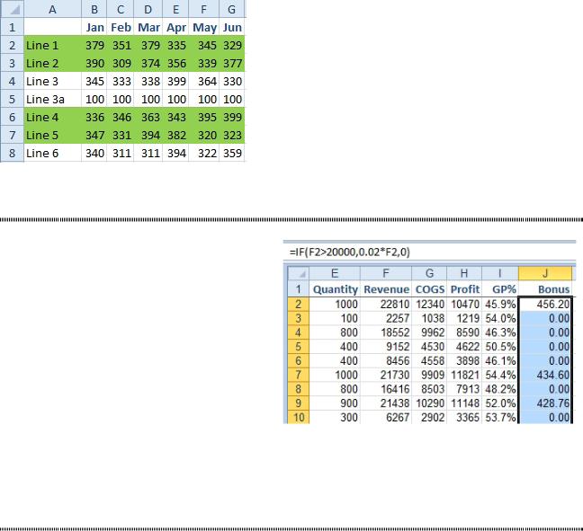
Problem: My VP of Sales announced that we are paying a 2% bonus for all sales over $20,000 this month. How do I calculate the bonus?
Strategy: Use the IF function. The function has three arguments. The first argument is a logi- cal test. This is any expression that will result in a value of TRUE or FALSE. For example,
F2>20000 is a logical test. The next argument is a formula that should be used if the logical test is true. The final argument is a value or formula to be used when the logical test is not true. The for- mula =IF(F2>20000,0.02*F2,0) can be thought of
in these words, “If the revenue in F2 is greater Figure 370 An IF function calculates the bonus. than 20,000 then 2% of F2, otherwise 0.”
Additional Details: The formula will not pay a bonus for someone who sold exactly $20,000. If such a sale should get a bonus, then use =IF(F2>=20000,0.02*F2,0).
IF WITH TWO CONDITIONS
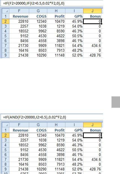
Problem: The CFO decided we should only pay the 2% bonus if a second condition is met. The GP% must be 50% or higher in addition to the sale being over $20,000.
Strategy: There are three common solutions to this problem: nesting IF statements, using AND, using boolean formulas. All three will be discussed here.
The most common solution is nesting one IF statement inside of another. The formula would be: =IF(F2> 20000,IF(I2>0.5,0.02*F2,0),0). This first checks if the revenue is over $20,000. The second argument holds a formula to use when the logical test is true. In this case, the second argument is another IF statement that checks to see if the GP% is over 50%.
PART 2: CALCULATING WITH EXCEL |
149 |
|
|
Figure 371 Using a second IF statement as the second argument.
Gotcha: Don’t forget to type the ,0) at the end of the formula. This will provide the third argument and closing parentheses for the first IF statement.
Imagine if you had to test for five conditions. The above approach becomes unwieldy, as the formula is =IF (Test1,IF(Test2,IF(Test3,IF(Test4,IF(Test5, Formula If True,0),0),0),0),0). Using AND will simplify the calculation.
The AND function will hold up to 255 logical tests. Separate each test with a comma. The AND function
will return TRUE if all of its arguments are TRUE. If any argument is false, then AND will return FALSE. 2 Use the AND() function as the logical test inside the IF statement. =IF(AND(F2>20000,I2>0.5),0.02*F2,0).
Figure 372 Using AND simplifies the IF statement.
If you see the power of AND, then you will appreciate the OR and NOT functions. The OR function takes up to 255 logical tests. If any one of the tests is TRUE, then OR will return TRUE.
The NOT function will reverse a TRUE to FALSE and a FALSE to TRUE. Students of logic design might remember that when you algebraically simplify a complex boolean expression, using NOT(OR()) might be the simplest way to create a test.
I’ve done my Power Excel seminars for thousands of people who use Excel 40 hours a week. 70% of those people suggest using multiple IF statements. 29.9% of those people suggest using AND. Only one person has ever suggested the following clever method.
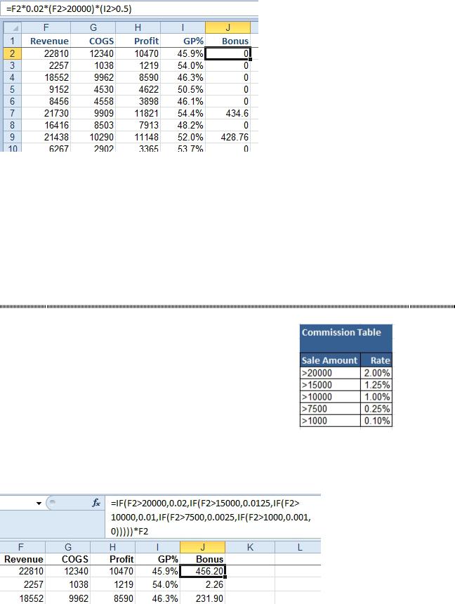
This formula starts out calculating a 2% bonus for everyone: =F2*0.02. But then the formula continues with two additional terms. =F2*0.02*(F2>20000)*(I2>.5). Those additional terms must be in parentheses. Excel treats (F2>20000) as a logical test and will evaluate that expression to either TRUE or FALSE. As Excel is calculating the formula, one intermediate step will be =22810*0.02*TRUE*FALSE.
When Excel has to use TRUE or FALSE in an calculation, the TRUE is treated as a one. The FALSE is treated as a zero. Since any number times zero is zero, the logical tests at the end of the formula will wipe out the bonus if any one of the conditions is not true. =22810*0.02*1*0 becomes 0. In row 7, =21730*0.02*1*1 becomes $434.60 and a bonus is paid.
150 |
POWER EXCEL WITH MR EXCEL |
|
|
Figure 373 Multiplying by a logical test is equivalent to AND.
Additional Details: Excel treats TRUE as a 1 when you use an operator such as +-*/^ on the TRUE value. This does not happen when Excel is calculating functions. If you enter =SUM(A1:E1) and cells in that range contain a TRUE, the TRUE is ignored.
Gotcha: Don’t use this last method when you have an OR condition. Traditionally, AND is equivalent to multiplication and OR is equivalent to addition. While the multiplication concept works fine in Excel, the addition will end up paying a double-bonus: =F2*0.02*((Test1)+(Test2)) might end up with =F2*0.02*2 which is not what you want.
See Also: Learn to Use Boolean Logic Facts to Simplify Logic
TIERED COMMISSION PLAN WITH IF
Problem: I am calculating a commission based on a sliding scale. The rate is based on the size of the sale, using the table shown here.
Strategy: You can solve this with several IF statements or with the unusual form of the VLOOKUP function.
To use the IF function, it is important that you start looking for the largest category first. Say that a cell contains a sale of $21,000. Checking for F2>20000 would return a TRUE, but checking for F2>1000 would be TRUE as well. You need to start checking for the largest value. If the sale is not larger than that value, then move on to checking for smaller values.
Figure 374 Sales above $15K and less than $20K are paid at 1.25%.
In the formula below, the IF function is finding the correct rate. The result of the IF function is multiplied by the revenue in F2. This prevents you from having to enter *F2 five different times in the formula.
Figure 375 Five IF statements nested together.
The formula is =IF(F2>20000,0.02,IF(F2>15000,0.0125,IF(F2>10000,0.01,IF(F2>7500,0.0025,IF(F2>100 0,0.001,0)))))*F2.
PART 2: CALCULATING WITH EXCEL |
151 |
|
|
As the commission plan becomes more complex, you would have to keep adding more IF statements. The current limit is 32 IF statements nested together. As recently as Excel 2003, the limit was 7 IF statements. It does not take long before this method becomes unwieldy.
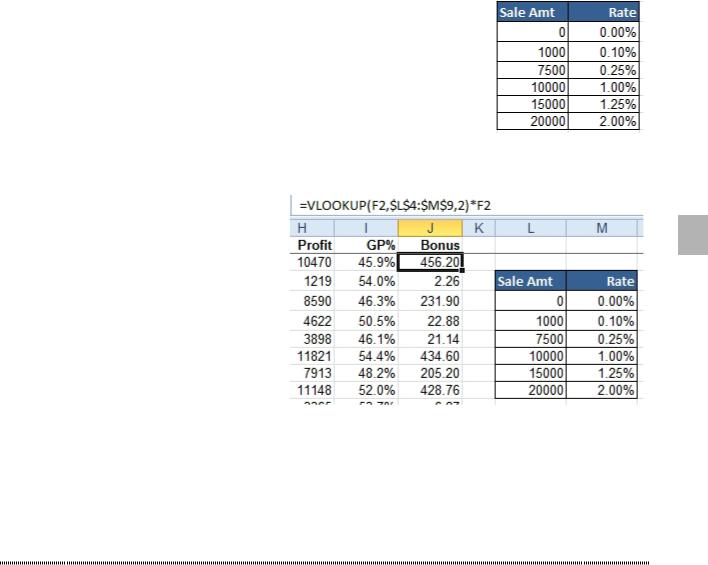
You’ll be learning more about VLOOKUP after about 15 more topics. Most VLOOKUP formulas in this book end with a FALSE to indicate a close match. Here is one case where a VLOOKUP that omits the FALSE can save the day.
To use a VLOOKUP, you have to reverse the order so that the largest lookup value appears at the end of the table. Add a beginning row with zero to handle the sales smaller than $1000. (Actually, depending on how you handle negative values, the negative values might need to be first.)
Figure 376 Lookup table where the values go from smallest to largest.
In the table above, a sale of $5000 is not found in the table. Using a typical VLOOKUP with
FALSE at the end would result in an #N/A 2 error. When you leave off the FALSE, Excel
will look for the value that is just smaller than 5000. In this case, it will return the 0.10% since 1000 is the level just smaller than $5000.
Figure 377 Leave off FALSE. Lookup finds the just- smaller value.
Additional Details: You might some day have a situation where you need Excel to find the value in the table that is just larger. You can not do this with VLOOKUP, but you can do it with MATCH. The last argument in MATCH can be 0 for exact match, 1 for the value just lower or -1 for the value just higher. Combine MATCH with INDEX to replicate a range-lookup where you want the just-higher value.
DISPLAY UP/DOWN ARROWS
Problem: I have a series of closing stock prices. If the price for the day goes up, I want to display an up symbol. If the price goes down, display a down symbol.
Strategy: Use an IF statement in combination with a Webdings or Wingdings font.
Most computers have at least four font faces composed of symbols. To easily browse the symbols, enter
=CHAR(ROW()) in cells A1:A256. Change the font for column A to Webdings or one of the three Wingdings fonts. As you browse through the symbols and see one that you would like, click on the symbol. Below is a possible arrow to use. You can see that this is in the Wingdings 3 font. From the row number, you know it is character code 199. From the formula bar, you can see that it is the C with a cedilla mark below.
152 |
POWER EXCEL WITH MR EXCEL |
|
|
Figure 378 Character 199 is a possibility.
If you are reading this and you have a Portuguese keyboard, you probably have a key with the cedilla C.
However, you will have to fly to France to find an E with a grave accent. You could try to master the art of holding down Alt while typing 0199 on the numeric keypad, or you could use CHAR(199).
Personally, for me, all of those are too much hassle and I won’t use the arrows shown above. Instead, I found the symbols that correspond to letters on my keyboard, so that I can easily type them in the formula.
Figure 379 These six symbols are all typeable on a U.S. keyboard.
The strategy is to write an IF statement that produces a 5 for positive and a 6 for negative. Then, format those cells to use the
Webdings font.
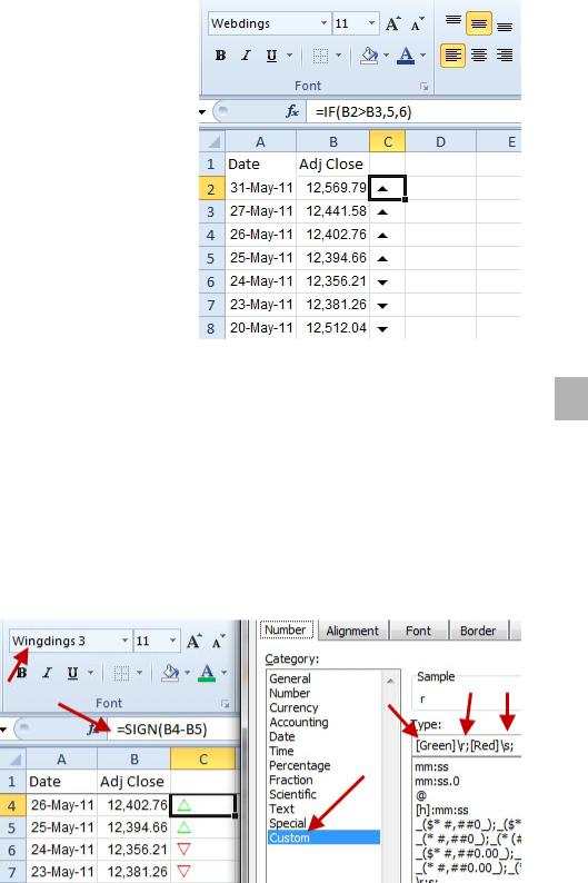
Use a formula such as =IF(B2>B3,5,6) to use the Webdings symbols. If you prefer the filled triangles from Wingdings 3, use =IF(B2>B3,”p”,”q”). Initially, you will get a column of 5 and 6.
Figure 380 The formula produces 5’s and 6’s.
Select column C and change the font to Webdings. Use Left alignment.
PART 2: CALCULATING WITH EXCEL |
153 |
|
|
Figure 381 Convert the column to Wingdings. |
|
Gotcha: If you ever need to edit the formula in C, it will appear in Webdings font and be unreadable in |
2 |
the cell. Use the Formula bar to see the real formula. |
If you want to display the arrows in green and red, change the font color of column C to green. Then use
Home, Conditional Formatting, Highlight Cells Rules, Equal to, 5. Open the Format dropdown and choose
Custom Format. On the Font tab, choose a bright red.
While Wingdings is a cool technique, an easier way to display Up/Down Arrows is "Use the SIGN Function for Up/Flat/Down Icon Set" on page 470
Alternate Strategy: You can avoid the IF statement and use a custom number format. Use a formula of =SIGN(B2-B3) in column C. This will return a negative one for days that the price went down, positive one for days when the price went up, and a zero for days where the price is unchanged.
Change the custom number format to [green]\r;[red]\s;. Change the font to Wingdings 3.
Figure 382 Forcing Excel to show r for positive and s for negative.
The custom number format is using three zones. The first zone is showing a lower case r in green for any positive number. The second zone is showing a lower case s in red for any negative number. The third zone is indicated by the final semi-colon and is blank, indicating no symbol for zero values. When you convert column C to Wingdings 3, you get the arrows shown.