


WHY DOES OFFICE 365 HAVE BETTER FEATURES?
Problem: I have TEXTJOIN and Funnel Charts at home, but not at work, What is going on?
Strategy: You have Office 365 at home. Buy agreeing to pay a monthly or annual fee for Office, you are getting frequent updates and new features. Microsoft is at war with the I.T. departments who still want to buy Office the old way. If someone buys Office 2016, they get a few new features, but they will never get the new monthly features. The days of the annual Service Pack are gone.
In the good old days (2003, 2007, 2010, 2013), Microsoft would spend three years putting new features into Office and the customers would invest $400 every other release. Now, Microsoft wants you to rent your copy of Office. Pay $10, $12, or $15 a month or $99 a year and you will get monthly updates.
I originally said that I would never rent Office. But then Microsoft started putting must-have features in Office 365 and not in the regular release of Office, so now I can see that renting Office 365 is the only logi- cal choice.
With Office 365, you will get to use mobile versions of Excel on an iPad, iPhone or Android device.
WHICH VERSION OF OFFICE 365 HAS POWER PIVOT?
Problem: The Office 365 website is super-confusing. I don’t want to buy the wrong version.
Strategy: If you want Power Pivot and all options of Power Query, you need to go with the $12 a month Pro Plus plan or the $15 a month E3 plan. Surprisingly, the $12.50 Small Business plan does not have Power Pivot. And, in an incredibly short-sighted move, the University edition does not have Power Pivot. If you don’t think you will ever need Power Pivot, then the $10 a month Home edition will allow you to install Excel on five computers.
WHY DO I HAVE TO SIGN IN TO EXCEL?
Problem: What is the deal with signing in to Office? Any why do they want my Flickr info in Excel?
Strategy: Even if you are not using Office 365 to subscribe to Office, Excel will ask you to store your Of- fice account information in the File, Account pane. This is not some attempt to harvest e-mails so they can spam you about the next MrExcel Power Excel seminar. There are actually good things that happen when you sign in on all of your computers:
●● Recent files that you save to OneDrive will appear in the recent list of all of your computers. If you were working on a file at work and save it to the cloud, it will be available when you get home. No more forgetting the USB drive at the office.
●● Ribbon customizations are carried through to all of your computers.
Saving your Flickr information allows you to Insert, Online Pictures and easily add photos that you’ve uploaded to the file sharing sites. Twitter, LinkedIn, and Facebook information was used in Excel 2013 to allow posting a workbook to social networks. That feature never caught on and was removed from Excel
2016.
3
4 |
POWER EXCEL WITH MR EXCEL |
|
|
|
HOW CAN I USE EXCEL ON DUAL MONITORS? |
Problem: Why is it so hard to use Excel on two monitors?
Strategy: This problem is fixed in Excel 2013. Every Excel workbook gets its own window, complete with a ribbon and formula bar. Open two workbooks, drag on to the other monitor and you will have 36 linear inches of Excel.
In Excel 2010, you have to use this hack:
●● Force Excel 2010 to open a second instance of Excel. You can hold down the Shift key while opening
Excel to create a second instance of Excel. Downside: you can not copy formulas from one instance to the other.
HOW CAN I OPEN THE SAME WORKBOOK TWICE?
Problem: I used to open two copies of the same workbook. I could select cells in copy B, see the total in the status bar, and then type that information in to a different place in copy A. Now that Excel 2013 opens every workbook in a new window, I can not open the same workbook twice.
Strategy: Open the first instance of the workbook. Then, force Excel to open in a new instance by hold- ing down the Shift key while opening Excel. In the second instance of Excel, use File, Open to open the workbook again.
FIND ICONS ON THE RIBBON
Problem: I know a certain feature exists in Excel, but I can not find it in the Ribbon.
Strategy: Use the new Tell Me feature in Excel 2016. Located to the right of the last tab in the Ribbon, a box with a lightbulb and “Tell Me What You Want To Do” appears. Click in the box and type the name of the feature. A selectable list of commands appears.
Figure 4 These commands are usually hidden in Commands Not in the Ribbon, but are now available.
Gotcha: If you are in Excel 2013 and don’t have Tell Me, open an Excel workbook at Office.Live.Com and use the Tell Me command in Excel Online.
WHERE IS FILE, EXIT?
Problem: What happened to the old Exit command?
Strategy: Although Exit is missing from the File menu in 2013-2016, you can use Alt+F, X to invoke the Exit command. Or, add Exit to the Quick Access Toolbar.
1. The top-left corner of Excel contains a tiny strip with icons for Save, Undo, and Redo. Right-click that strip and choose Customize Quick Access Toolbar.
2. The top left dropdown starts with Popular Commands. Open that dropdown and choose All Com- mands. You now have an alphabetical list of 2000+ commands.
3. Scroll through the list to find Exit. When you find your command, click the command. Click the Add>> button in the center of the screen to add the command to the Quick Access Toolbar.
PART 1: THE EXCEL ENVIRONMENT |
|
5 |
|
|
|
|
WHERE ARE MY MACROS? |
|
Problem: Did Microsoft abandon the macro facility? Where are the buttons to record a new macro, run a macro, and so on? How do I get to the Visual Basic Editor?
|
Strategy: Most of the macro icons are hidden. Three macro options appear on |
|
|
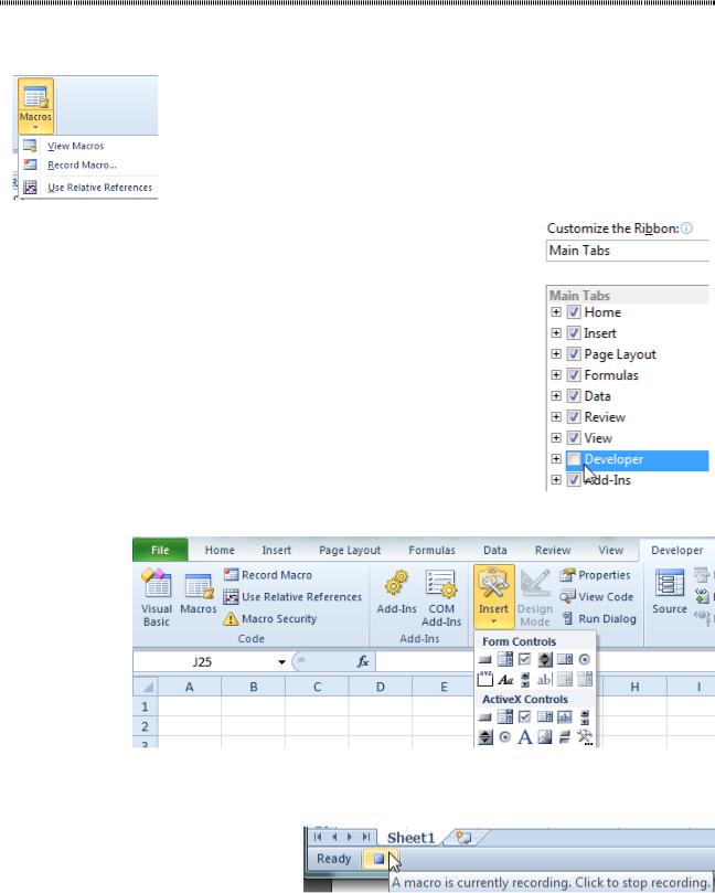
the extreme right end of the View tab. You use the Macros dropdown to view |
|
|
macros, record a macro, or use relative references while recording a macro. |
|
|
To access the rest of the macro functionality, you need to enable a hidden De- |
|
|
veloper ribbon tab. Choose File, Options, Customize Ribbon. Add a checkmark |
|
|
next to Developer. The Developer tab offers macro commands, buttons from the |
|
Figure 5 A subset of |
former Forms toolbar and Control Toolbox, and XML settings. |
|
|
|
|
macro commands are |
|
|
available on the View |
|
1 |
tab. |
|
|
|
|
|
Figure 6 Microsoft disable the Developer tab by default.
Figure 7 If you use macros, enable the Developer tab.
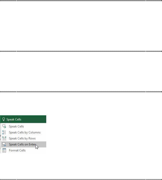
Additional Details: When you are recording a macro, instead of seeing the Stop Recording icon floating above the Excel window, you now see it in the Status Bar, next to Ready.
Figure 8 Once you’ve recorded a macro, the Stop and Record buttons will appear next to Ready.
The same area of the status bar includes a Record Macro button when you are not recording a macro.
However, because there is not a Relative References button, you cannot effectively record macros without using either the View tab or the Developer tab of the ribbon.
6 |
POWER EXCEL WITH MR EXCEL |
|
|
|
CUSTOMIZING THE RIBBON |
Problem: I want to customize the ribbon.
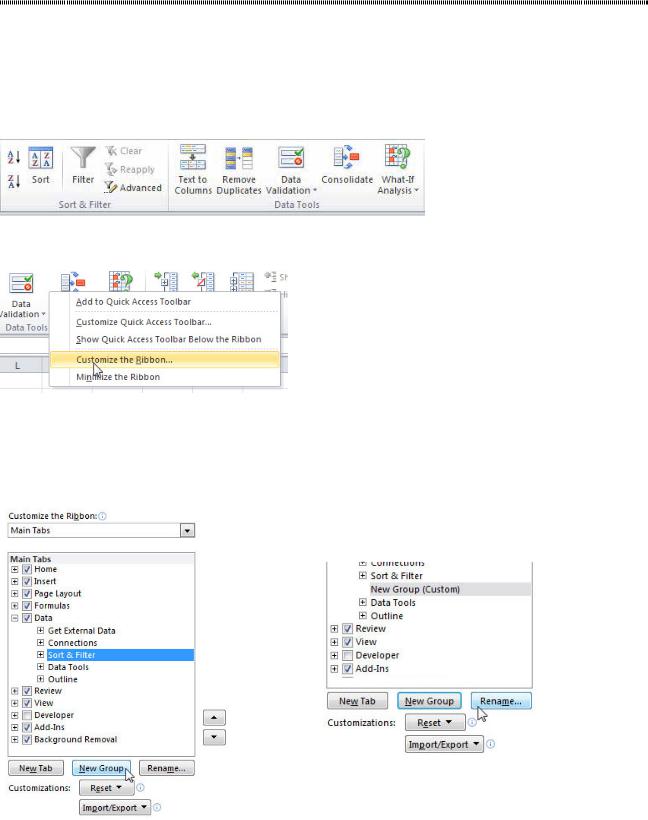
Strategy: Ribbon customizations in Excel 2013/2016 are weak compared with the customization capabili- ties in Excel 2003. You might feel like the Pivot Table command belongs on the Data tab rather than on the Insert tab. You can add a new group to the Data tab to hold the pivot table icons.
First, look at the ribbon and decide where you want the new group to appear. Perhaps a good location would be between the Sort & Filter group and the Data Tools group.
Figure 9 Decide where you want the new group to appear.
Right-click anywhere on the ribbon and choose Customize the Ribbon.
Figure 10 Right-click the ribbon to access this menu.
The Customize dialog contains two large list boxes. You will first be working with the list box on the right side of the screen. Expand the plus sign next to the Data entry to see the groups on the Data tab. If you want a new group to appear after the Sort & Filter group, click Sort & Filter, and then click the New Group button below the list box.
Excel adds a new group with the name of New Group
(Custom). Click the Rename button below the list box.
Figure 11 Choose where the new group should go.
Figure 12 Choose to rename the group
Type a new name in the Rename dialog. Also, choose an icon. This icon will appear only when the Excel window gets small enough to force the group into a dropdown, as shown later in Figure 17..
PART 1: THE EXCEL ENVIRONMENT |
7 |
|
|
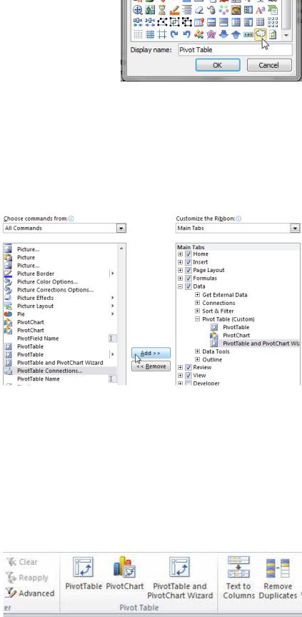
Figure 13 Type a new name and choose an icon to represent the group. |
|
|
Note: The 180 icons available are a far cry from the 4096 icons available in Excel 2003. As I pointed out at |
|
|
the beginning of this chapter, toolbar customization took a giant step backward after Excel 2003. |
|
|
After renaming the new group in the list box on the right side, it is time to turn your attention to the list |
|
|
box on the left side. It starts out showing Popular Commands. Use the dropdown above the left list box to |
|
|
change from Popular Commands to All Commands. |
|
|
Scroll down to the commands starting with Pivot. You will see a confusing array of commands. Click the |
|
|
1 |
||
first PivotTable icon, and click the Add button in the center of the screen. Click the second PivotChart icon, |
||
|
||
and then click the Add button. Click PivotTable and PivotChart Wizard, and then click the Add button. |
|
|
|
Figure 14 Choose icons to add to the new group.
It is sometimes difficult to figure out which icons you want. There are two icons that say PivotTable. The first icon is simply an icon. The second icon is an icon with a rightward-facing triangle on the right side of the list box. That triangle indicates that the second icon is actually a dropdown that leads to more choices. That second PivotTable dropdown icon is the icon at the bottom half of the Insert tab’s Pivot Table group.
It opens to enable you to choose between PivotTable and PivotChart. You might prefer to use that icon instead.
Two PivotChart icons are available. Hover over each icon to see that the first one is the PivotChart icon available on the PivotTable Tools Options tab. You will also see that the second icon is the one on the In- sert tab. The first PivotChart icon will be grayed out unless you are in a pivot table. The second PivotChart icon is the one that is used to create a new pivot chart from a data set.
This figure shows the resulting group on the Data tab.
Figure 15 The custom group is added to the ribbon.
If you are wondering why you had to choose an icon back in Figure 13, it is for people who have the Excel window resized to a narrower width. If you make your Excel window narrower, the custom group will even- tually get squished down to a single dropdown. Your icon will appear on that dropdown, as shown here.