

- •Table of Contents
- •About the Author
- •Dedication
- •Foreword
- •Acknowledgments
- •Why Does Office 365 Have Better Features?
- •Which Version of Office 365 Has Power Pivot?
- •Why Do I Have to Sign in to Excel?
- •How Can I Use Excel on Dual Monitors?
- •How Can I Open The Same Workbook Twice?
- •Find Icons on the Ribbon
- •Where is File, Exit?
- •Where Are My Macros?
- •Customizing the Ribbon
- •Go Wide
- •Minimize the Ribbon to Free Up a Few More Rows
- •Use a Wheel Mouse to Scroll Through The Ribbon Tabs
- •Why Do The Charting Ribbon Tabs Keep Disappearing?
- •Use Dialog Launchers For More Choices
- •Icon, Dropdowns, and Hybrids
- •Zoom is at the Bottom
- •Make Your Most-Used Icons Always Visible
- •The Excel 2003 Alt Keystrokes Still Work (If You Type Them Slowly Enough)
- •Use Keyboard Shortcuts to Access the Ribbon
- •Why Do I Have Only 65,536 Rows?
- •Which File Format Should I Use?
- •Why Does The File Menu Cover The Entire Screen?
- •How Do I Close The File Menu?
- •Increase the Number of Workbooks in the Recent Files List
- •Change All Print Settings in Excel
- •I Just Want The Old Print Preview Back
- •Get Quick Access to Formatting Options Using the Mini Toolbar
- •What Is Protected Mode?
- •Use a Trusted Location to Prevent Excel’s Constant Warnings
- •My Manager Wants Me to Create a New Expense Report from Scratch
- •Open a Copy of a Workbook
- •Open Excel with Ctrl+Alt+X
- •Have Excel Always Open Certain Workbook(s)
- •Set up Excel Icons to Open a Specific File on Startup
- •Use a Macro to Customize Startup
- •Control Settings for Every New Workbook and Worksheet
- •Excel Says I Have Links, But I Can Not Find Them
- •Automatically Move the Cell Pointer After Enter
- •Return to the First Column After Typing the Last Column
- •Enter Data in a Circle (Or Any Pattern)
- •How to See Headings as You Scroll Around a Report
- •How to See Headings and Row Labels as You Scroll Around a Report
- •Why is the Scrollbar Slider Suddenly Tiny?
- •Why Won’t My Scrollbar Scroll to My Charts?
- •Jump to the Edge of the Data
- •Jump to Next Corner of Selection
- •Ctrl+Backspace brings the Active Cell into View
- •Zoom with the Wheel Mouse
- •Copy a Formula to All Data Rows
- •A Faster Way To Paste Values
- •Quickly Turn a Range on Its Side
- •Quickly Rearrange Rows Or Columns
- •Quickly Copy Worksheets
- •Use Group Mode to Change All Worksheets
- •Find Text Numbers
- •Why Can’t Excel Find a Number?
- •Mix Formatting In A Single Cell
- •Enter a Series of Months, Days, or More by Using the Fill Handle
- •Have the Fill Handle Fill Your List of Part Numbers
- •Teach Excel to Fill A, B, C
- •Add Total to the End of Jan, Feb, ... Dec
- •Put Date & Time in a Cell
- •Use Excel as a Word Processor
- •Add Excel to Word
- •Use Hyperlinks to Create an Opening Menu for a Workbook
- •Spell check a Region
- •Stop Excel from AutoCorrecting Certain Words
- •Use AutoCorrect to Enable a Shortcut
- •Why Won’t the Track Changes Feature Work in Excel?
- •Simultaneously Collaborate on a Workbook with Excel Web App
- •How to Print Titles at the Top of Each Page
- •Print a Letter at the Top of Page 1 and Repeat Headings at the Top of Each Subsequent Page
- •How to Print Page Numbers at the Bottom of Each Page
- •How to Make a Wide Report Fit to One Page Wide by Many Pages Tall
- •Add a Printable Watermark
- •Print Multiple Ranges
- •Add a Page Break at Each Change in Customer
- •Save My Worksheet as a PDF File
- •Send an Excel File as an Attachment
- •Save Excel Data as a Text File
- •Close All Open Workbooks
- •I Just Closed an Unsaved Workbook
- •Roll Back to an AutoSaved Version
- •Have Excel Talk to You
- •Enter Special Symbols
- •What Do All the Triangles Mean?
- •Why does Excel Insert Cell Addresses When I Edit In a RefEdit Box?
- •F4 Repeats Last Command
- •Print all Excel Keyboard Shortcuts
- •Create a Personal Macro Workbook
- •Macro to Toggle Positive to Negative
- •Assign a Macro to a Shortcut Key
- •Assign a Macro to a Toolbar Icon
- •Use a Macro to Change Case to Upper, Lower, or Proper
- •Get Free Excel Help
- •Start a Formula with = or +
- •Three Methods of Entering Formulas
- •Why Does Excel 2013 Look Like A Slot Machine?
- •Use Parentheses to Control the Order of Calculations
- •Long Formulas in the Formula Bar
- •Copy a Formula That Contains Relative References
- •Copy a Formula While Keeping One Reference Fixed
- •Create a Multiplication Table
- •Calculate a Sales Commission
- •Simplify the Entry of Dollar Signs in Formulas
- •Learn R1C1 Referencing to Understand Formula Copying
- •Create Easier-to-Understand Formulas with Named Ranges
- •See All Named Ranges at 39% Zoom
- •Use Named Constants to Store Numbers
- •Total Without Using a Formula
- •Add or Multiply Two Columns Without Using Formulas
- •Type 123 to Enter 1.23
- •Join Two Text Columns
- •Concatenate Several Cells
- •Join Text with a Date or Currency
- •Break Data Apart Using Flash Fill
- •Parse Data using Text to Columns
- •Excel Is Randomly Parsing Pasted Data
- •I Lose Leading Zeroes From CSV Files
- •Open CSV File With Dates in D/M/Y Format
- •Handle Dates in YYYYMMDD format
- •My G/L Software Uses a Trailing Minus for Negative Numbers
- •Parse Data With Leader Lines
- •Parse Multi-Line Cells
- •Change Smith, Jane to Jane Smith
- •Convert Numbers to Text
- •Fill a Cell with Repeating Characters
- •CLEAN Hasn’t Kept Up With The Times
- •Add the Worksheet Name as a Title
- •Use AutoSum to Quickly Enter a Total Formula
- •AutoSum Doesn’t Always Predict My Data Correctly
- •Use the AutoSum Button to Enter Averages, Min, Max, and Count
- •Ditto The Formula Above
- •The Count Option of the AutoSum Dropdown Doesn’t Appear to Work
- •Total the Red Cells
- •Automatically Number a List of Employees
- •Automatically Number the Visible Rows
- •Discover New Functions Using the fx Button
- •Get Help on Any Function While Entering a Formula
- •Use F9 in the Formula Bar to Test a Formula
- •Quick Calculator
- •When Entering a Formula, You Get the Formula Instead of the Result
- •Highlight All Formula Cells Using Conditional Formatting
- •You Change a Cell in Excel but the Formulas Do Not Calculate
- •Calculate One Range
- •Why Use the Intersection Operator?
- •Understand Implicit Intersection
- •Find the Longest Win Streak
- •Add B5 On All Worksheets
- •Consider Formula Speed
- •Exact Formula Copy
- •Calculate a Loan Payment
- •Calculate Many Scenarios for Loan Payments
- •Back into an Answer Using Goal Seek
- •Create an Amortization Table
- •Do 40 What-if Analyses Quickly
- •Random Walk Down Wall Street
- •What-If For 3 Or More Variables
- •Rank Scores
- •Round Numbers
- •Round to the Nearest $0.05 with MROUND
- •Round Prices to the Next Highest $5
- •Round 0.5 towards Even Per ASTM-E29
- •Separate the Integer From the Decimals
- •Why Is This Price Showing $27.85000001 Cents?
- •Calculate a Percentage of Total
- •Calculate a Running Percentage of Total
- •Use the ^ Sign for Exponents
- •Raise a Number to a Fraction to Find the Square or Third Root
- •Calculate a Growth Rate
- •Find the Area of a Circle
- •Figure Out Lottery Probability
- •Help Your Kids with Their Math
- •Convert Units
- •XOR Only Works Correctly for Two Values
- •Find the Second Largest Value
- •Format Every Other Row in Green
- •\Use IF to Calculate a Bonus
- •IF with Two Conditions
- •Tiered Commission Plan with IF
- •Display Up/Down Arrows
- •Stop Showing Zeroes in Cell Links
- •Count Records That Match a Criterion
- •Build a Table That Will Count by Criteria
- •Sum Records That Match a Criterion
- •Can the Results of a Formula Be Used in SUMIF?
- •Calculate Based on Multiple Conditions
- •Avoid Errors Using IFERROR
- •Use VLOOKUP to Join Two Tables
- •Every VLOOKUP Ends in False
- •Lookup Table Does Not Have to Be Sorted
- •Beware of #N/A from VLOOKUP
- •Add New Items to the Middle Of Your Lookup Table
- •Consider Naming the Lookup Table
- •Remove Leading and Trailing Spaces
- •Your Lookup Table Can Go Across
- •Copy a VLOOKUP Across Many Columns
- •INDEX Sounds Like an Inane Function
- •You Already Know MATCH, Really!
- •INDEX Sounds Like an Inane Function - II
- •VLOOKUP Left
- •Fast Multi-Column VLOOKUP
- •Speed Up Your VLOOKUP
- •Return the Next Larger Value in a Lookup
- •Two-Way Lookup
- •Combine Formulas into a Mega-Formula
- •Combine Two Lists Using VLOOKUP
- •Watch for Duplicates When Using VLOOKUP
- •Return the Last Entry
- •Return the Last Matching Value
- •Sum All of the Lookups
- •Embed a Small Lookup Table In Formula
- •I Don’t Want to Use a Lookup Table to Choose One of Five Choices
- •Is there Something More Flexible than CHOOSE?
- •Lookup Two Values
- •Add Comments to a Formula
- •Create Random Numbers
- •Randomly Sequence a List
- •Play Dice Games with Excel
- •Generate Random Without Repeats
- •Calculate a Trendline Forecast
- •Forecast Data with Seasonality
- •Build a Model to Predict Sales Based on Multiple Regression
- •Switching Columns into Rows Using a Formula
- •SUM a Range that is C5 Rows Tall Using OFFSET
- •Replace Volatile OFFSET with INDEX
- •How Can You Test for Volatility?
- •Whatever Happened to the @@ Function?
- •Tables Are Like a Database in Excel
- •Dealing with Table Formulas
- •Rename Your Tables
- •Charts , VLOOKUP & Pivots Expand With The Table
- •Before Deleting a Cell, Find out if Other Cells Rely on It
- •Calculate a Formula in Slow Motion
- •Which Cells Flow into This Cell?
- •Color all Precedents or Dependents
- •Monitor Distant Cells
- •Auditing Worksheets with Inquire
- •Use Real Dates
- •How Can I Tell If Have Real Dates?
- •Convert Text Dates to Real Dates
- •Format Dates
- •Format Dates As Quarters or Weeks
- •Display Monthly Dates
- •Add a Column to Show Month or Weekday
- •Calculate First of Month
- •Calculate the Last Day of the Month
- •Calculate Invoice Due Dates
- •Calculate Receivable Aging
- •NOW, or TODAY?
- •Find the Last Sunday Of the Month
- •Calculate Work Days
- •Calculate Work Days for a Farmers Market
- •Calculate Age in Years, Months, Days
- •Coerce an Array of Dates from 2 Dates
- •Use Real Times
- •Strangeness of Time Formatting
- •Convert Time to Decimal Hours
- •Calculate with Time
- •Enter Minutes and Seconds
- •Convert Text to Time
- •Can Excel Track Negative Time?
- •Fill Blanks With Value Above
- •See Formulas in Excel 2013
- •Create a Bell Curve in Excel
- •Change from Lower to Upper Case in Excel
- •Spell Out Numbers in Excel
- •Copy Macro Code from the Internet Into an Add-In
- •Return Data from a Webservice in Excel 2013
- •Add New Functions to Excel with Fast Excel SpeedTools Extras
- •=SUM(B1:B5) is Better Than =B1+B2+B3+B4+B5
- •How to Set up Your Data for Easy Sorting and Subtotals
- •How to Fit a Multiline Heading into One Cell
- •No Tiny Blank Columns Between Columns
- •How to Sort Data
- •Sort Days of the Week
- •Sort a Report into a Custom Sequence
- •Sort All Red Cells to the Top of a Report
- •Sort Pictures With Data
- •Quickly Filter a List to Certain Records
- •Use Search While Filtering
- •Filter by Selection
- •Use AutoSum After Filtering
- •Filter Only Some Columns
- •Find the Unique Values in a Column
- •Use Advanced Filter
- •Replace Multiple Filter Criteria with a Single Row of Formulas
- •Add Subtotals to a Data set
- •Use Group & Outline Buttons to Collapse Subtotaled Data
- •Manually Apply Groups
- •Group Report Sections
- •Copy Just Totals from Subtotaled Data
- •Sort Largest Customers to the Top
- •Select 100 Columns in Subtotals
- •Enter a Grand Total of Data Manually Subtotaled
- •Add Other Text to the Subtotal Lines
- •Subtotals by Product Within Region
- •Format the Subtotal Rows
- •My Manager Wants a Blank Line After Each Subtotal
- •Subtotal One Column and Count Another Column
- •Can You Get Medians?
- •Horizontal Subtotals
- •Be Wary
- •Send Error Reports
- •Help Make Excel Better
- •Remove Blank Rows from a Range
- •Remove Blanks from a Range While Keeping the Original Sequence
- •Double Space Your Data Set
- •Use Find to Find an Asterisk
- •Use an Ampersand in a Header
- •Hide Zeros & Other Custom Number Formatting Tricks
- •Use Consolidation to Combine Two Lists
- •Combine Four Quarterly Reports
- •Find Total Sales by Customer by Combining Duplicates
- •Remove Duplicates
- •Preview Remove Duplicates Without Removing Them
- •Protect Cells That Contain Formulas
- •Find Differences In Two Lists
- •Number Each Record, Starting at 1 for a New Customer
- •Deal with Data in Which Each Record Takes Five Physical Rows
- •Add a Customer Number to Each Detail Record
- •Use a Built-in Data Entry Form
- •Cell AutoComplete Stopped Working
- •Data Cleansing with Flash Fill in Excel 2013
- •Flash Fill was there and is now Gone
- •Flash Fill Was Not Perfect
- •Flash Fill Won’t Fill Numbers
- •Flash Fill and Dates
- •Flash Fill and Ambiguous Data
- •Use a Pivot Table to Summarize Detailed Data
- •Your Manager Wants Your Report Changed
- •Add or Remove Fields from an Existing Pivot Table
- •Summarize Pivot Table Data by Three Measures
- •Why Does the Pivot Table Field List Keep Disappearing?
- •Move or Change Part of a Pivot Table
- •See Detail Behind One Number in a Pivot Table
- •Use Multiple Value Fields as a Column or Row Field
- •Update Data Behind a Pivot Table
- •Why do I Get a Count Instead of a Sum?
- •Convert Your Data to a Table Before Adding Records
- •Create a Flattened Pivot Table for Reuse
- •Replace Blanks in a Pivot Table with Zeros
- •Collapse and Expand Pivot Fields
- •Specify a Number Format for a Pivot Table Field
- •Preserve Column Widths
- •Show Yes/No in a Pivot Table
- •Pivot Table Format Defaults
- •Format Pivot Tables with the Gallery
- •None of the 46,273 Built-In Styles Do What My Manager Asks For
- •Select Pivot Table Parts For Formatting
- •Apply Conditional Formatting to a Pivot Table
- •Can I Save Formatting in a Template?
- •Manually Re-sequence the Order of Data in a Pivot Table
- •Present a Pivot Table in High-to-Low Order by Revenue
- •Excel 2016 Sometimes Auto-Groups Daily Dates to Month
- •Group Daily Dates by Month in a Pivot Table
- •Create a Year-Over-Year Report
- •Group by Week in a Pivot Table
- •Limit a Pivot Report to Show Just the Top 5 Customers
- •Build a Better Top Five Using Groups
- •Build a Better Top Five with A Filter Hack
- •Build a Better Top 5 Using the Data Model
- •Limit a Report to Just One Region
- •Create an Ad-Hoc Reporting Tool
- •Create a Report for Every Customer
- •Create Pivot Charts
- •Add Visual Filters to a Pivot Table or Regular Table
- •Run Many Pivot Tables From one Slicer
- •Filter Dates Using a Timeline in Excel 2013 & Newer
- •Group Employees Into Age Bands
- •Create a Frequency Distribution
- •Grouping 1 Pivot Table Groups Them All
- •Reduce Size 50% Before Sending
- •Drag Fields to the Pivot Table
- •Create a Report That Shows Count, Min, Max, Average, Etc.
- •Better Calculations with Show Values As
- •Pivot Ranks Don’t Match RANK()
- •Calculated Fields in a Pivot Table
- •Add a Calculated Item to Group Items in a Pivot Table
- •Group Text Fields to Build Territories
- •Calculations Outside of Pivot Tables
- •Show Customer Account & Name
- •Show Months with Zero Sales
- •Create a Unique List of Customers with a Pivot Table
- •Use a Pivot Table to Compare Two Lists
- •Use a Pivot Table When There Is No Numeric Data
- •Fix Misspelled Customer Names
- •Create a Pivot Table from Access Data
- •What Happened to Multiple Consolidation Ranges in Pivot Tables?
- •What are the Products in Power BI And How Can I Get Them?
- •Know if You Have 32-Bit or 64-Bit Excel
- •Load and Clean Data with Power Query
- •Power Query is Easier to Learn than VBA Macros
- •I Have More than 1,048,576 Rows of Data
- •Load a List of File Names into Excel
- •Load a Folder of CSV Files into a Single Excel Worksheet
- •My Headings Repeat Every 60 Rows
- •Fill in Blanks with Values from Above
- •Use Power Query to Clean Data Already in Excel
- •Pivot from Multiple Tables in Excel 2013 Data Model
- •Reporting from the Smaller Side of the Relationship
- •Use Joiner Tables Between Tables
- •Five Reasons to Use Power Pivot
- •Why Isn’t Power Pivot Tab in the Ribbon?
- •Get Excel Data Into Power Pivot
- •Open the Power Pivot Window
- •Define Relationships Between Tables
- •Sort Month Name by Month Number
- •Create a Calendar Table
- •The Formulas are called DAX
- •Adding Calculations In the Power Pivot Grid
- •Refer to a Related Table in a Formula
- •Creating the Power Pivot Table
- •Building the Pivot Table
- •Feature X Won’t Work in Power Pivot
- •Replace Calculated Fields with DAX
- •Calculate() is Like SUMIFS()
- •Unapply a Filter Using DAX
- •Unfilter Using Time Intelligence
- •Convert Power Pivot to Formulas
- •January Actuals and February Plan
- •Power View Is Replaced with Power BI
- •Power BI Transforms Excel Data into Interactive Dashboards
- •First POwer BI Step: Get a Free Account for Power BI
- •Optional Step 1: Take the Sample Dashboards for a Spin
- •Use Q&A to Investigate Your Data
- •Click a Dashboard Element to Open the Underlying Report
- •Click in one Chart to Filter Other Charts
- •Enable Drill-Down Mode
- •Sorting is Hidden Behind More Options
- •Optional Step 2: Connect to an Existing Service
- •Download Power BI Desktop to Your Computer
- •Prepare Your Excel Data for Power BI
- •Add a Calendar Table
- •Three Icons in Power BI Desktop
- •In Power BI Desktop, the Power Query Tools Are Called Get Data
- •Load Your Excel Data to Power BI Desktop
- •In Power BI Desktop, the Power Pivot tools are called Modeling
- •Define Relationships in Power BI Desktop
- •Classify Your Geography Fields in Power BI Desktop
- •Prevent Power BI from Adding Up Year Fields
- •Sort This by That
- •Define Synonyms in Power BI Desktop
- •Hide Columns So They Can't Be Chosen
- •Three Ways to BUild Visualizations in a Report
- •FOrmatting a Chart
- •Add Lines using Analytics
- •Adding More Visualizations to a Page
- •It is Insanely Easy to Build a Hierarchy
- •Open Source Visualizations
- •Every Chart is a Slicer For Other Charts
- •A Report Can Have Multiple Pages
- •Using Maps in Power BI Desktop
- •Three Types of Filters
- •Where is the Top 10 Filter?
- •Add Titles, Logos, & Embelishments
- •Don't Forget to Save Your File!
- •Share Your Dashboard to Power BI in the Cloud
- •Use Quick Insights
- •View Your Report in a Browser
- •Q&A Works on Dashboards, Not Reports
- •Share a Dashboard With Your Manager
- •Wait a Second - a Sharing Link? Isn't this Dangerous?
- •Consume Your Dashboard Using Power BI Mobile
- •What Does All Of This Cost?
- •How Do I Update My Dashboard Every Day?
- •That's All For Power BI In This Book
- •Put a Pivot Table on a Map In Excel 2013 Power Map
- •Tricks for Navigating the Map in Power Map
- •Fine-Tuning Power Map
- •Creating a Video from Power Map
- •Use an Alternate Map for Power Map
- •Filtering in Power Map
- •Excel Data to Mailing Labels in Word
- •Excel 2013 Allows Slicers on Regular Tables
- •Use Power Query to Load Many Web Pages
- •Create a Chart with One Click
- •Teach Excel Your Favorite Chart
- •Move a Chart
- •Copy a Chart Detached from the Data
- •Add New Data to a Chart
- •Excel 2013 Offers Easy Chart Formatting
- •Begin Excel 2010 Formatting on Design
- •The Chart Layout Tab Is Missing in Excel 2013
- •Formatting Charts in Excel 2010 with Layout
- •Legend At the Top
- •The 2010 Format Dialog Box is a Task Pane in 2013
- •Display an Axis in Millions
- •Select Anything on a Chart to Format
- •The Format Dialog Box Offers a New Trick
- •Use Meaningful Chart Titles
- •Avoid 3-D Chart Types
- •Prevent the Drop to Zero
- •Explode One Slice of the Pie
- •Move Small Pie Slices To Second Chart
- •Add a Trendline to a Chart
- •See Detail on Large & Small Data Points
- •Chart Two Series with Differing Orders of Magnitude
- •Hide Subtotals From Chart in Excel 2013
- •Create Pivot Charts from Detail Data in Excel 2013
- •Use Formulas for Chart Labels in Excel 2013
- •Interactive Chart to Show One Customer
- •Tie the Chart Title to a Cell
- •Excel 2016 Adds a Waterfall Chart
- •Use an Invisible Series to Float Columns
- •Use Rogue Series for Shading
- •Two Stacked, One Clustered Column
- •Conditional Format a Chart
- •Scatter Charts are Versatile But Require a Different Workflow
- •When do I Use Which Chart Type?
- •Track Sales Leads with a Funnel Chart
- •Create Tiny Charts with Sparklines
- •Sparklines Are Not Scaled Together
- •What is the Win Loss Sparkline For?
- •Labeling Sparklines
- •Shade the Normal Range in a Sparkline
- •Convert a Table of Numbers to a Visualization
- •Control Values for Each Icon
- •Add Icons to Only the Good Cells
- •Use the SIGN Function for Up/Flat/Down Icon Set
- •Data Bars Options
- •Comparative Histogram
- •Select Every Kid in Lake Wobegon
- •There is a Font Optimized for Excel
- •Show Checkmarks in Excel
- •Add Bullets to Excel
- •Use the Border Tab in Format Cells
- •Remove Borders from Filled Cells
- •Double Underline a Grand Total
- •Why Did the Colors Change in Excel 2013?
- •Where Are My Excel 2003 Colors?
- •Transform Black-and-White Spreadsheets to Color by Using a Table
- •Fit a Slightly Too-Large Value in a Cell
- •Turn Off Wrap Text in Pasted Data
- •Delete All Pictures in Pasted Data
- •Prevent Long Text from Spilling
- •Show Two Values in a Split Cell
- •For Each Cell in Column A, Have Three Rows in Column B
- •Show Results as Fractions
- •Better Scientific Notation
- •Fill a Cell with Asterisks
- •I type 152 and get 1.52
- •Use Cell Styles to Change Formats
- •Move Columns by Sorting Left to Right
- •Move Columns Using Insert Cut Cells
- •Move Rows or Columns with Shift Drag
- •Select All Cells Using the Keyboard
- •Change the Width of All Columns with One Command
- •Copy Column Widths to a New Range
- •Copy Row Heights
- •Use White Text to Hide Data
- •Hide Values Using a Number Format
- •Hide and Unhide Data
- •Group Columns Instead of Hiding Them
- •Hide Error Cells When Printing
- •Unhide All Sheets
- •Very Hide a Worksheet
- •Organize Your Worksheet Tabs with Color
- •Copy Formatting to a New Range
- •Copy Without Changing Borders
- •Power Up Format Painter
- •Fill Formatting
- •Change All Red Font Cells to Blue Font
- •Replace Partially Bold Cells
- •Change the Look of Your Workbook with Document Themes
- •Create Your Own Theme
- •Bring Back the Office 2010 Colors And Shiny Objects
- •Change the Background of a Worksheet
- •Add a Printable Background to a Worksheet
- •Remove Hyperlinks Automatically Inserted by Excel
- •Select a Hyperlink Cell Without Following the Hyperlink
- •Pasted URLs Don’t Become Hyperlinks
- •Debug Using a Printed Spreadsheet
- •Change the Appearance of Cell Comments
- •Control How Your Name Appears in Comments
- •Force Some Comments to ALWAYS Be Visible to Provide a Help System
- •Change the Comment Shape to a Star
- •Add a Pop-up Picture of an Item in a Cell
- •Add a Pop-up Picture to Multiple Cells
- •Build Reports Where Columns in Each Section 1 Don’t Line Up
- •Paste a Live Picture of a Cell
- •Add Formatting to Pictures in Excel
- •Remove Picture Background
- •Inserting a Screen Clipping
- •Draw an Arrow to Visually Illustrate That Two Cells Are Connected
- •Add Connectors to Join Shapes
- •Circle a Cell on Your Worksheet
- •Draw Perfect Circles
- •Add Text to Any Closed Shape
- •Place Cell Contents in a Shape
- •Rotate a Shape
- •Create Dozens of Lightning Bolts
- •Make a Logo into a Shape
- •Draw Business Diagrams with Excel
- •Choose the Right Type of SmartArt
- •Use the Text Pane to Build SmartArt
- •Change a SmartArt Layout
- •Format SmartArt
- •Switch to the Format Tab to Format Individual Shapes
- •Use Cell Values as the Source for SmartArt Content
- •Add WordArt to a Worksheet
- •Chart and SmartArt Text Is Automatically WordArt
- •Excel 2013 Offers an Excel App Store
- •Add a Dropdown to a Cell
- •Configure Validation to “Ease up”
- •Use Validation to Prevent Duplicate Data Entry
- •Use Validation to Create Dependent Lists
- •Add a ToolTip to a Cell to Guide the Person Using the Workbook
- •Combine Validation with AutoComplete
- •Afterword
- •Index
144 |
POWER EXCEL WITH MR EXCEL |
|
|
t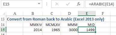 Figure 359 Convert from Roman back to Arabic.
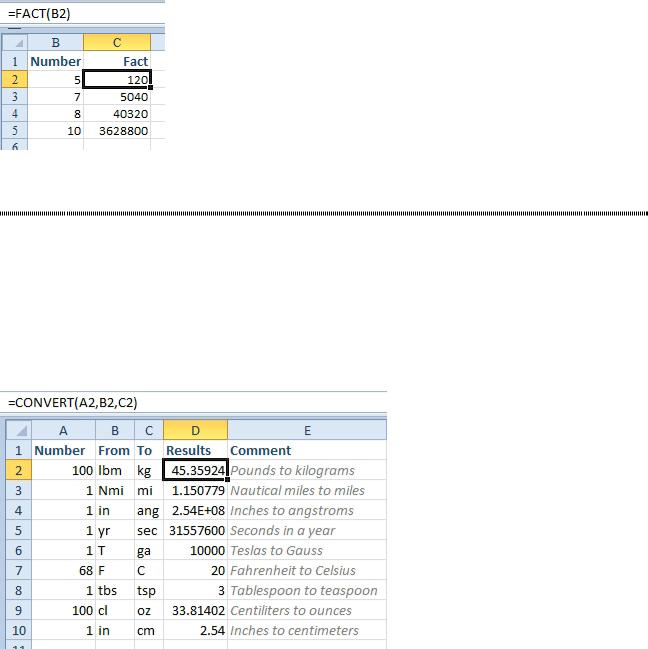
Factorials: The last obscure function you need to help with the math homework is the factorial function, FACT. A factorial is a number multiplied by every integer between itself and 1. To write 5 factorial, you use the number followed by an exclamation point. So, for example, 5! is 5 x 4 x 3 x 2 x 1, or 120. Use =FACT(5) to calculate 5!.
Figure 360 The factorial of 5 is 5 x 4 x 3 x 2 x 1, or 120.
CONVERT UNITS
Problem: I need to convert units of measure. I can never remember that there are .453 kilograms in a pound or 2.54 centimeters in an inch.
Strategy: You can use the CONVERT function to convert a certain number of one unit to another unit.
The CONVERT function works with units of weight, distance, time, pressure, force, energy, power, magnetism, temperature, and liquid measure.
The syntax for this function is =CONVERT(number, from unit, to unit). It’s important that you use the correct abbreviations (for example, lbm for pounds mass), so look in Excel help if you need to.
This figure shows a sampling of the conversions possible with this function.
Figure 361 CONVERT handles many conversion factors.
PART 2: CALCULATING WITH EXCEL |
145 |
|
|
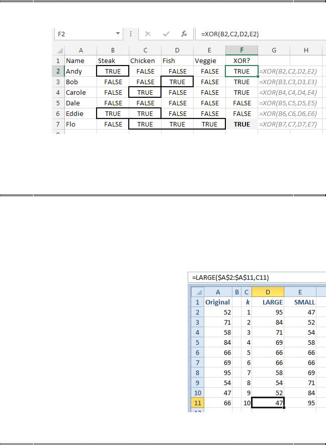
XOR ONLY WORKS CORRECTLY FOR TWO VALUES
Problem: Excel 2013 introduced an Exclusive OR (XOR) function. It won’t work correctly for more than two values.
Figure 362 Flo ordered three items, but XOR incorrectly returns TRUE. |
|
Strategy: Blame it on Electrical Engineers. They use XOR chips in circuits. Despite it’s name, the XOR |
|
chip counts if an odd number of inputs are TRUE. The Excel team decided to emulate the chip instead of |
|
English. To truly do what all non-EE’s understand to be XOR, you could use =COUNTIF(B7:I7,True)=1. |
2 |
|
|
|
|
FIND THE SECOND LARGEST VALUE
Problem: I can find the largest and smallest numbers using MAX and MIN. I am trying to identify the largest and smallest three numbers. How can I find the second largest number?
Strategy: Use the LARGE or SMALL functions. These functions take a range of values, then a k value. If you use a k value of 1, the LARGE function is exactly like a MAX: =LARGE(B2:B100,1). The real value in LARGE is the ability to ask for the second largest value using =LARGE(B2:B100,2).
In the figure below, you can see the LARGE and SMALL for an entire set of 10 data points. Note that 66 is reported as both the 5th and 6th largest value due to two 66 entries in the original data set.
Figure 363 Use LARGE and SMALL to return the kth largest value.
FORMAT EVERY OTHER ROW IN GREEN
Problem: Got any cool uses for MOD? Got any old-school methods for applying the greenbar format that was in the Excel 2003 AutoFormat dropdown?
146 |
POWER EXCEL WITH MR EXCEL |
|
|
Strategy: This topic is about an out-of-the-box method for using MOD to apply a format. If the only goal was to apply alternate-row shading, you could use any of these methods:
●● Alt+O+A and choose the Excel 2003 format. ●● Ctrl+T, choose Banded Rows and any format.
●● Leave row 2 unformatted. Fill row 3 with green. Select row 2 & row 3. Use the fill handle to drag to the bottom of the data set. Open the Paste Options menu and choose Fill Formatting Only.
However, this topic is going to use math to do the formatting.
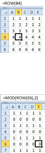
Consider the ROW function. =ROW(A2) will return 2 because A2 is in the second row of the worksheet. Here is a big range of ROW functions.
Figure 364 The ROW function tells you the row number.
Now, imagine taking all of those row numbers and dividing by 2. Throw away any integer result, but keep the remainder. This is a strange thought. All of the even number rows will not have a remainder at all. For the odd number rows, say that you take seven divided by 2. You get 3 with a remainder of 1. Throw out the 3 and keep only the remainder. The MOD function will give you only the remainder. =MOD(ROW(A7),2) will return a 1 because 7 divided by 2 has a remainder of 1. The next figure shows the MOD formula for several rows. Notice that you get stripes of 0’s and 1’s.
Figure 365 MOD of the ROW, 2 will return stripes.
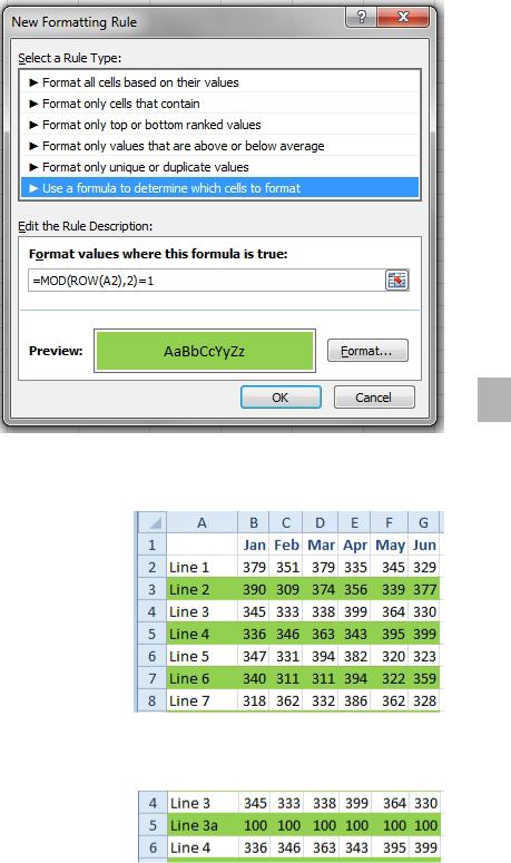
So, how do you use this formula to add a green stripe in every other row? You do it with old-school conditional formatting. Follow these steps.
1. Select your range of data. Perhaps it is A2:G900.
2. Make a note of which cell is the active cell. This is the cell address that is shown in the Name box, to the left of the formula bar. You will need this cell address in step 4.
3. Select Home, Conditional Formatting, New Rule.
4. There are six types of rules listed in the top of the New Formatting Rule dialog. Choose the last type, called Use A Formula To Determine Which Rows To Format. When you choose this type, a formula bar appears in the bottom of the dialog. It is called Format Values Where This Formula is True.
5. Click in that formula box. Type a formula similar to this formula, but use the cell address from step
2 instead of A2. =MOD(ROW(A2),2)=1.
6. Click the Format… button.
7. On the Fill tab, choose a fill color. Click OK.
PART 2: CALCULATING WITH EXCEL |
147 |
|
|
2
Figure 366 Your dialog should look like this one.
8. Click OK to apply the rule.
The range will be filled with an every-other row format.
Figure 367 Greenbar format.
The cool part is that if you delete a row or insert a row, the MOD(ROW(),2) formulas will recalculate and the shading will redraw. In the figure below, Line 3a is now green and Line 4 is white.
Figure 368 The formatting recalcs after inserting rows.
Additional Details: With a little math reasoning, you can change the format pattern. What if you wanted the even rows to be formatted? Change the formula to =MOD(ROW(A2),2)=0. If you wanted two rows of green followed by two rows of white, use =MOD(ROW(A2),4)>1.