

36 |
POWER EXCEL WITH MR EXCEL |
|
|
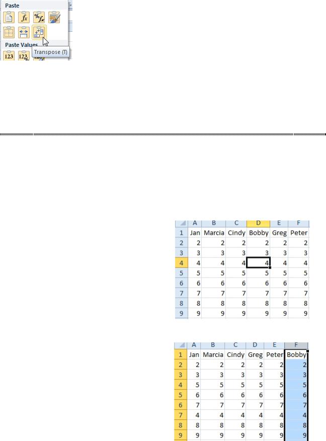
Figure 77 Use this icon to turn the pasted data sideways.
Gotcha: The columns you paste to will not automatically resize to fit the data. To fix this problem, you can select the appropriate range (in this case, C1:Z1) and then choose Home, Format, AutoFit Column Width.
Additional Details: You can use Transpose to convert a horizontal row of numbers into a column. In ad- dition, you can use it to turn a rectangular range on its side.
QUICKLY REARRANGE ROWS OR COLUMNS
Problem: I want to move row 5 to appear after row 7. I don’t want to sort. I don’t want to insert a new row, copy, paste, delete the old row. What is the fastest way?
Strategy: This topic will cover some little-known shortcut keys.
●● Shift+Spacebar selects the entire row. ●● Ctrl+Spacebar selects the entire column.
●● Shift+Drag Border will insert the selected range in a new spot. ●● Ctrl+Plus Sign will insert cells above or to the left
●● Ctrl+Minus sign will delete the selection.
Here is an example. Say that you want to move row
4 after row 7 and that you want to move Bobby after Peter.
1. Select the whole row using Shift+Spacebar.
2. Hold down the shift key. Drag the lower border of the selection and drop it below row 7.
3. Select a cell in D. Select the whole column using Ctrl+Spacebar.
4. Shift+Drag the right border of the selection after column F.
Figure 78 You want to rearrange this data.
If you wanted to delete column B, select one cell in
B, Ctrl+Spacebar to select the whole column, then
Ctrl+Minus to delete.
Figure 79 Shift-drag the selection to move it.
PART 1: THE EXCEL ENVIRONMENT |
|
37 |
|
|
|
|
QUICKLY COPY WORKSHEETS |
|
Problem: I’ve created the perfect report for January. I’ve formatted the column widths. I’ve changed the
Page Setup. I have custom views. I need to make copies of the report for February through December in the current workbook.
Strategy: You need the Move or Copy command. Normally, you would right-click the January worksheet tab, choose Move or Copy, choose New Book, Create a Copy, OK. However, there is a faster way.
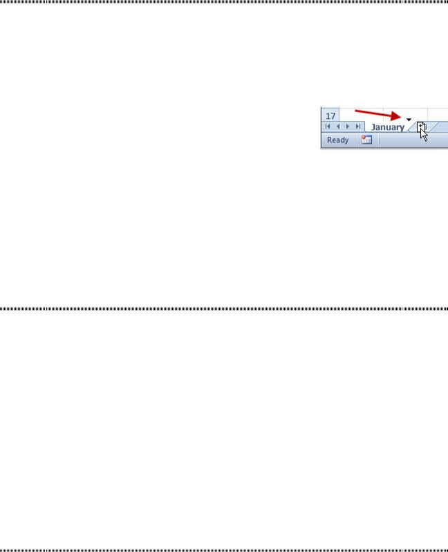
While holding down the Ctrl key, drag the January worksheet tab and drop it to the right of the January tab.
Figure 80 Ctrl+Drag the tab to make a copy. |
|
|
1 |
||
Watch the black triangle pointer. The worksheet copy will be added where the indicator appears. |
||
|
||
Gotcha: The name for the new worksheet will be January (2). Double-click the worksheet name and type |
|
|
a new name. |
|
|
If you make five copies of January, you can select January through June by selecting January and then |
|
|
Shift+Clicking on June. Ctrl+Drag January and drop after June to make copies for July through Decem- |
|
|
ber. You will still have to manually rename all of the worksheets. |
|
|
Additional Details: If you have two workbooks opened and use View, Arrange, Vertical, you can Ctrl+Drag |
|
|
a worksheet from one workbook to another. |
|
USE GROUP MODE TO CHANGE ALL WORKSHEETS
Problem: I now have 12 nearly identical worksheets. I have to make a similar change to all 12 sheets.
Strategy: Use Group Mode. Any changes you make to the active sheet will apply to all of the sheets in the group.
●● If you need to put all of the sheets in the workbook in group mode, you can right-click any tab and choose Select All Sheets.
●● To group several consecutive sheets, select the first sheet, then shift-click on the last sheet. Alterna- tively, use Ctrl+Shift+PageDown to add sheets to the right to the group.
●● To group sheets that are not adjacent, select the first sheet, then Ctrl+Click other sheets.
When worksheets are grouped, you will see the word [Group] to the right of the workbook name in the title bar. Any changes that you make will happen to all of the sheets in the group.
Gotcha: Don’t get distracted and forget that you are in group mode. I’ve forgotten that I was in group mode and spent an hour keying numbers into January, only to discover that I was destroying numbers on all of the back sheets.
Additional Details: There are three ways to exit group mode. First: Right-click any sheet tab and choose
Ungroup Sheets. Second: If a sheet is not included in the group, select that sheet. Third option: If all of the sheets are included in the group, click on any sheet that is not the active sheet.
FIND TEXT NUMBERS
Problem: I suspect that there are cells in my data that contain text numbers instead of numbers. I know that numbers entered as text cause a variety of problems. For example, although a formula such as
=E3+E4 will include the text number in E3, most functions, such as SUM or AVERAGE, will ignore the text cells. Text versions of a number will sort to a different place than numeric versions. If I use a MATCH or VLOOKUP function, a text version of 3446 will not match a numeric version of 3446. How can I find text entries that need to be converted to numbers?
38 |
POWER EXCEL WITH MR EXCEL |
|
|
Strategy: These text cells, as well as a variety of other potential errors, are noted by a dark green triangle in the upper-left corner of the cell. As shown below, cells C6, E2, E3, E6, and E7 have triangles in their upper-left corners because they are text entries that look like numbers.
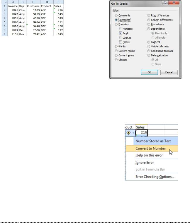
Figure 81 Some cells contain text that looks like numbers.
Instead of looking for those little triangles, here’s an easier way to locate all the text entries so you can convert them to numbers:
1. Select the entire range of data by selecting one cell and then pressing Ctrl+*.
2. Select Home, Find & Select, Go To Special. Excel will display the Go To Special dialog.
3. Select Constants. Deselect the options Numbers,
Logicals, and Errors, leaving only Text selected.
Figure 82 Choose Constants. Deselect
Numbers.
Results: All the text entries will be highlighted.
Additional Details: There are a number of ways to convert these cells from text to numbers. The easiest way is to get all the text cells in one contiguous range. If you can sort the data by column E descending, all the text entries will sort to the top of the list.
You can convert a contiguous range of text numbers. To do so, you use the Error (exclamation point) dropdown and select Convert to
Number. This method works only if the top-left cell in your selection contains a number stored as text.
For earlier versions of Excel, you can use the following trick: 1. Enter a zero in a blank cell.
2. Copy the cell with the zero by using Ctrl+C. 3. Highlight the text cells.
4. Choose Edit, Paste Special. In the Paste Special dialog that appears, select Values and Add and then click OK.
Adding a zero to the text cells will cause them to be converted to real numbers.
Figure 83 Open the error dropdown to convert text to numbers.
Alternate Strategy: The fastest way to convert a column of numbers to text is to select the column and type Alt+DEF (that is, Alt+D followed by E then F). This little command uses the default Text to Columns settings which will convert your text to numbers.
WHY CAN’T EXCEL FIND A NUMBER?
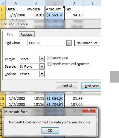
Problem: The Excel Find and Replace dialog drives me crazy. I always have to go to the Options button to specify that it should look in Values. In the figure below, the mouse pointer is showing the value that Excel says is not there is actually there. Why can’t Excel find a number?
PART 1: THE EXCEL ENVIRONMENT |
39 |
|
|
1
Figure 84 Psst, Excel! Try looking under the mouse pointer.
Strategy: You’ve pointed out a lot of the problems with Find and Replace. Let’s take a quick review to uncover some of the problems. First, when you select Home, Find & Select, Find, Excel presents the sim- plified version of the Find and Replace dialog without the important settings shown at the bottom of the figure above.
There are important settings hiding behind the Options button. These settings will often cause a Find to fail. Say that you have a calculation for sales tax in column D. Cell D3 shows 70.81 as the result of a for- mula. By default, Excel is searching the formulas instead of the values. If you tried Find without changing
Formulas to Values, it will not find $70.81.
Searching the text of the formulas is a bit annoying. How often do you say to yourself, “Wow, I wonder in which cell I used the SQRTPI function?” But even more annoying are the other settings, such as Match
Case and Match Entire Cell Contents. These settings can be useful, but if you happened to change them at 8:04 a.m. today and haven’t closed Excel since then, even though you’ve opened and closed 40 other workbooks and are working on something completely different, Excel will remember that previous setting.
You will often get stung by a strange setting left behind earlier in the day, or even a setting changed when a macro tried to use the Find command with Match Entire Cell Contents turned on.
So why can’t Excel see the 1354.80 value in Figure 84? Excel is displaying cell C16 with a currency sym- bol and a comma, and in order to find the cell, you have to search for $1,354.80! Because Excel’s forte is numbers, it’s rather disappointing that Excel works like this. But when you understand it, you can work around it.
Additional Details: People often ask how they can search through all sheets in a workbook. You do this by changing the Within dropdown from Sheet to Workbook.
Additional Details: Amazingly, Excel can find cells that are displaying as number signs (#) instead of numbers. Say that you have a column where 5% of the numbers are showing as #####.
Now, any sane person would make the column wider or turn on Shrink to Fit, but Excel allows you to per- form the following rather crazy set of steps:
1. Select the range of numbers. Press Ctrl+F to display the Find dialog.