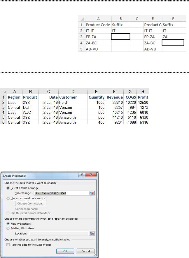
Problem: How will Flash Fill get this right? Even I wouldn’t know what to fill in next?

Strategy: Before invoking Flash Fill with Ctrl+E, provide enough examples to establish the pattern. If you invoke Flash Fill from B3, you will get the pre- fix instead of the suffix. By filling in one more example and running Flash Fill from I4, you will get the suffix.

Figure 755 Give Flash Fill enough examples.

USE A PIVOT TABLE TO SUMMARIZE DETAILED DATA

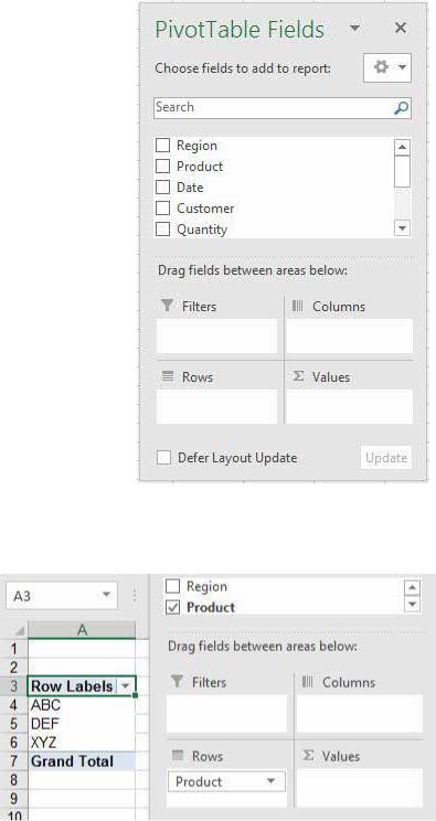
Problem: I have many rows of sales data. I want to produce a summary report that shows sales by region and product.

Figure 756 Summarize this data set.

Strategy: To solve this problem, you can use a pivot table. As Excel’s most powerful feature, pivot tables are well suited to this type of analysis.

Creating a summary of revenue by region and product requires four mouse clicks and one mouse drag: 1. Ensure that your data is in list format and that every heading is unique. (For a refresher on list

format, see "How to Set up Your Data for Easy Sorting and Subtotals" on page 233.) 2. Select a single cell in the database. Select Insert, Pivot Table.

3. Excel’s IntelliSense will guess the range of your data. Ensure the range is correct and click OK.

Figure 757 Make sure that Excel guessed the correct range.

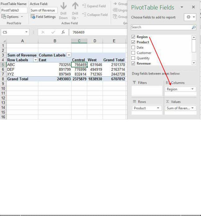
You will now see an empty pivot table icon, two new PivotTable Tools tabs on the ribbon, and the Pivot- Table Fields dialog.

The PivotTable Fields dialog includes a list of the fields at the top and four drop zones at the bottom of the dialog.

Note: The dialog is usually docked to the right side of the screen. For this book, I’ve undocked it so I can show the Pivot Table Fields next to the pivot table. Gotcha: It is difficult to redock the PivotTable Fields dialog. You have to grab the left side of the title bar and drag it 90% off the right edge of the Excel window.

Way back in Excel 2003, you would drag fields from the

Field List dialog to the pivot table. This process was frus- trating for people new to pivot tables. Now, you drag fields from the top of the Field List dialog to the proper drop zone at the bottom of the Field List dialog. In many cases, click- ing the field in the Field List dialog will move it to the cor- rect drop zone. In this case, you want to have products going down the side of the report and regions going across the top.

4.Click the Product check box in the top of the Field List dialog. Excel automatically moves it to the Row Labels drop zone. The pivot table shows a list of unique products in column A.

Figure 759 Click a text field, and Excel moves it to the Row area.

5. Click the Revenue check box in the top of the Field List dialog. Because this field is numeric, Excel will add it to the Values section of the pivot table.

6. If you click the Region check box, Excel will add it to the row area of the pivot table. Because you want regions to go across the top of your pivot table, drag the Region field from the top of the Field

List dialog and drop it in the Column Labels drop zone at the bottom of the Field List dialog.

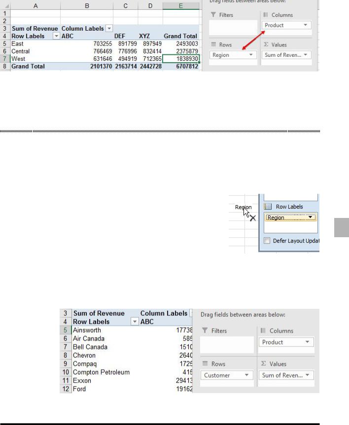
Figure 760 Checkmark Revenue, drag Region.

Excel will summarize the data by product and region, as shown above.

Additional Details: Pivot tables offer many powerful options. This topic describes the steps to create your first pivot table; you should read the next several topics to learn more about pivot tables.

Gotcha: If you were a pivot table pro in previous Excel versions, you can quickly adapt to the new pivot tables. The drop zones have been renamed. The Row Area drop zone is now Row Labels. The Column Area drop zone is now Column Labels. The Page Field drop zone is now Report Filter. The Data Area drop zone is now ∑ Values (although I will call it the Values drop zone, leaving off the ∑ symbol).

Gotcha: A dropdown at the top of the PivotTable Field List dialog offers five different views of the dialog. Three of those views omit either the fields or the drop zones. If your dialog box is missing one section, use the dropdown to return it to Fields Section and Areas Section Stacked. There are also views where the sec- tions are side by side. Throughout the next pages, I will refer to the drop zones at the bottom of the dialog.

If you have moved them to be side by side, then mentally change those instructions to read “the drop zones on the right side of the dialog.”

YOUR MANAGER WANTS YOUR REPORT CHANGED

Problem: I presented my first pivot table report, shown previously, to my manager. He said, “This is al- most perfect, but could you have the products going across the top and the regions going down the side?”

Strategy: Pivot tables make this change easy:

1. On the worksheet, select one cell within the pivot table. Excel will display the PivotTable Field List dialog.

2. In the dialog, drag the Region field from the Column Labels drop zone to the Row Labels drop zone. In this case, it does not matter if you drop the Region field above or below the Product field

3. In the dialog, drag the Product field from the Row Labels drop zone to the Column Labels drop zone.

Results: With two movements of the mouse, you have created a new report for your manager.

Figure 761 Move two fields to create a new report.

The first amazing feature of pivot tables is that they can summarize massive amounts of data very quickly.

This topic shows the second amazing feature: Pivot tables can be quickly changed to show another view of the data.

ADD OR REMOVE FIELDS FROM AN EXISTING PIVOT TABLE

Problem: I’ve seen how easy it is to rearrange an existing pivot table by swapping Region and Product fields. Now, what if I want to replace the Region field with the Customer field?

Strategy: In order to remove the Region field from a pivot table, you click on the Region button in the

Row Labels drop zone of the PivotTable Field List dialog. Then you drag the button outside the Field List dialog. The cell pointer will change to include a black X, which is synonymous with Delete. Or - simply uncheck Region in the top of the Pivot Table Fields dialog.

3

Figure 762 Remove a field.

To add the Customer field to the Row Labels drop zone, you simply click the Customer check box in the top of the PivotTable Field List dialog. Because the field is a text field, it will automatically move to the Row

Labels drop zone.

Results: The new field will be added to the pivot table.

Figure 763 Remove Region, add Customer.

SUMMARIZE PIVOT TABLE DATA BY THREE MEASURES

Problem: I want to summarize data by region, product, and customer. How can I use a two-dimensional report to show three dimensions of data?

Strategy: Several views of the data are possible. Say that you are starting with products across the top and customers down the side. From the top of the PivotTable Field List dialog, you click the Region field.

It is automatically added as the last row field. The view below shows the first customer and the purchases by region.

Figure 764 Regions within customer.

Another option is to drag the Region field heading above the Customer field heading in the bottom of the Field List dialog. Watch for the blue insertion bar.

If your mouse is not accurate enough to complete this drop, you can move the Product field to the Row Labels drop zone.

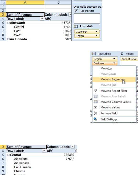
Then you open the dropdown arrow at the right side of the

Product field in the bottom of the Field List dialog and choose Move Up or Move to Beginning.

Figure 765 Drag fields, or use this drop- down menu.

Results: By changing the order of the fields in the row area, you now see the first region and all of the customers in that region.

Figure 766 Customers within region.

You can also stack fields in the Column Labels drop zone.