

272 |
POWER EXCEL WITH MR EXCEL |
|
|
Figure 699 New message when the answer is positive, negative, or zero.
Additional Details: There is a subtle difference between the 0 and # when used after the decimal point in a custom number format. A # indicates that Excel can display the digit if there is sufficient precision in the value. A 0 indicates that Excel must display the digit. The 0.000 format would cause 123.4 to display as 123.400 even though the last two digits are zero. The 0.0## format ensures that there is always one decimal place, but the second and third decimal places are used only if necessary.
Additional Details: To fill the white space before a number, precede the number format with two aster- isks. Similar to the security feature of old check printers, asterisks will appear before the number.
Figure 700 Custom format of **0.
Additional Details: You can use zeros before the decimal point to force Excel to display leading zeros.
The custom format 00000 will ensure that the zip code for Cambridge, Massachusetts, prints as 02142 instead of 2142. If you need a part number to appear as 4 digits, you can use the custom format 0000 to force leading zeros to appear.
USE CONSOLIDATION TO COMBINE TWO LISTS
Problem: Jerry and Tina each compiled sales figures from paper invoices. I need to combine Jerry and Tina’s list into a single list. Some customers are in both lists.
Figure 701 Combine the lists into a single list.
Strategy: Excel offers a great tool for consolidating data. Here’s how you use it:
1. Move the cell pointer to a blank area of the worksheet. You will need a blank area with several rows and a few columns.
2. Select Data, Consolidate.
3. Make sure that both boxes under Use Labels In are checked. This means that Excel relies on the headings to be the same and that the customer field is in the left column of each range.

PART 3: WRANGLING DATA |
273 |
|
|
4.Put the cell pointer in the Reference field. Click the Collapse button at the right end of the Reference field. With the mouse, select the first range: A1:B23. Click the Collapse button again to return to the
Consolidate dialog.
Note: There are times when you will want to consolidate just a single range of data. This would be effective if you needed to combine duplicate customers from one list. However, in this example, you need to combine two lists.
5. Click the Add button to move the first reference from the Reference field to the All References box. 6. After the first reference is added to the All References box, click the Collapse button again to specify
the second reference.
7. Use the mouse to select D1:E23. Click the Collapse button to return to the Consolidate dialog. Click the Add button to add the reference to the All References list. The Consolidate dialog should appear as below
3
.
Figure 702 Make sure both ranges are in the All References box.
8. Choose OK. In a few seconds, Excel will return a brand new list that extends down and to the right from your starting cell. The list will contain one instance of each customer along with the total revenue from the customer.
Figure 703 Excel combines the two lists into a single list.
Gotcha: The new list is not in any sequence. You can see that it kind of starts out in the sequence of the first list but then randomly inserts customers from the second list. You will probably want to sort the list alphabetically or by revenue. However, Excel always fails to fill in the label in the upper-left corner of the consolidation. If you want to sort the result, you need to type the word Customer in cell G2.
274 |
POWER EXCEL WITH MR EXCEL |
|
|
Additional Details: The Function box in the Consolidate dialog offers many functions other than SUM. For instance, if you want to find the largest purchase by each customer, you can use the MAX function.
Gotcha: The results of the consolidation are all static values. If you change an item in the original list, the consolidation will not automatically update. This is good because it allows you to delete the original two lists and keep just the new list.
COMBINE FOUR QUARTERLY REPORTS
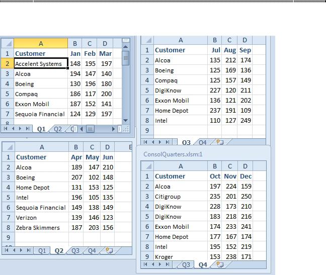
Problem: I have four worksheets for Q1 through Q4. Each worksheet has months across the top and cus- tomers down the side. The months and customers are not the same. I want to combine them into a single report.
Figure 704 Combine these four lists into a yearly report.
Strategy: The Consolidate command needs the row headings to be of the similar type, but not the exact same values. Consolidate will work here because column A in each worksheet contains customers (al- though not the same customers). Row 1 contains months (although not the same months).
1. Add a new worksheet named Year.
2. Select cell A1 on the Year worksheet.
3. Choose Data, Consolidate.
4. Click the Collapse button at the right end of the Reference box.
5. Browse to Q1. Select A1:D7. Click the icon at the right edge of the Reference box to return to the
Consolidate dialog.
6. Click the Add button in the Consolidate dialog. 7. Repeat steps 4-6 for Q2, Q3, and Q4.
8. Ensure Top Row and Left column are checked in the lower left corner of the Consolidate dialog. The dialog should look like this:

PART 3: WRANGLING DATA |
275 |
|
|
Figure 705 Choose a reference from each worksheet.
9. Click OK. You will have a report showing a superset of all customers and all months.
3
Figure 706 Excel consolidates the four quarters to one report.
10.Type Customer and press Enter to fill in the blank heading in A1.
11.Many empty cells appear in the consolidated data. This means that the customer did not have a record in that quarter. Select B2:M15. Press Ctrl+H to display Find & Replace. Leave the top box blank. Type 0 in the lower box. Click Replace All.
12.Sort the data by customer.
Additional Details: Make sure to add Q1 before Q2 and so on. The order of the months in row follows the order that the references were added.
Gotcha: There is a Browse button in the Consolidate dialog. This means that you can combine worksheets from different workbooks. However, the Browse button requires you to type the worksheet name and used range from memory without seeing the workbook. It would be much easier to open all four workbooks be- fore using Consolidate. You can use View, Switch Windows to move to another workbook while entering a reference.
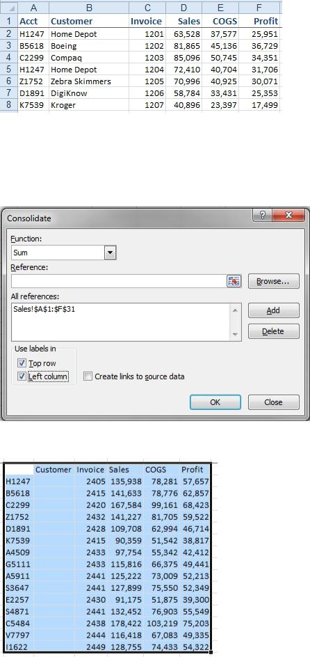
FIND TOTAL SALES BY CUSTOMER BY COMBINING DUPLICATES
Problem: I have an invoice register for the month. The report shows account, customer, invoice, sales, cost, and profit for each invoice. I want to combine customers in order to produce a report of sales by cus- tomer.
276 |
POWER EXCEL WITH MR EXCEL |
|
|
Figure 707 Consolidate the data to one row per customer.
Strategy: It is possible to consolidate a single list by using the labels in the left column. This will produce a report with one line per customer and totals of each numeric field. You can use data consolidation to solve this task:
1. Select a blank section of the worksheet. Select Data, Consolidate. In the Reference field, select the complete range of your data, including the headings. Ensure that the Left Column option is checked and that the Create Links to Source Data check box is unchecked. Click OK.
Figure 708 Specify a single range to consolidate.
Excel will combine all identical account numbers together.
Figure 709 One row per unique account number.