- •Table of Contents
- •About the Author
- •Dedication
- •Foreword
- •Acknowledgments
- •Why Does Office 365 Have Better Features?
- •Which Version of Office 365 Has Power Pivot?
- •Why Do I Have to Sign in to Excel?
- •How Can I Use Excel on Dual Monitors?
- •How Can I Open The Same Workbook Twice?
- •Find Icons on the Ribbon
- •Where is File, Exit?
- •Where Are My Macros?
- •Customizing the Ribbon
- •Go Wide
- •Minimize the Ribbon to Free Up a Few More Rows
- •Use a Wheel Mouse to Scroll Through The Ribbon Tabs
- •Why Do The Charting Ribbon Tabs Keep Disappearing?
- •Use Dialog Launchers For More Choices
- •Icon, Dropdowns, and Hybrids
- •Zoom is at the Bottom
- •Make Your Most-Used Icons Always Visible
- •The Excel 2003 Alt Keystrokes Still Work (If You Type Them Slowly Enough)
- •Use Keyboard Shortcuts to Access the Ribbon
- •Why Do I Have Only 65,536 Rows?
- •Which File Format Should I Use?
- •Why Does The File Menu Cover The Entire Screen?
- •How Do I Close The File Menu?
- •Increase the Number of Workbooks in the Recent Files List
- •Change All Print Settings in Excel
- •I Just Want The Old Print Preview Back
- •Get Quick Access to Formatting Options Using the Mini Toolbar
- •What Is Protected Mode?
- •Use a Trusted Location to Prevent Excel’s Constant Warnings
- •My Manager Wants Me to Create a New Expense Report from Scratch
- •Open a Copy of a Workbook
- •Open Excel with Ctrl+Alt+X
- •Have Excel Always Open Certain Workbook(s)
- •Set up Excel Icons to Open a Specific File on Startup
- •Use a Macro to Customize Startup
- •Control Settings for Every New Workbook and Worksheet
- •Excel Says I Have Links, But I Can Not Find Them
- •Automatically Move the Cell Pointer After Enter
- •Return to the First Column After Typing the Last Column
- •Enter Data in a Circle (Or Any Pattern)
- •How to See Headings as You Scroll Around a Report
- •How to See Headings and Row Labels as You Scroll Around a Report
- •Why is the Scrollbar Slider Suddenly Tiny?
- •Why Won’t My Scrollbar Scroll to My Charts?
- •Jump to the Edge of the Data
- •Jump to Next Corner of Selection
- •Ctrl+Backspace brings the Active Cell into View
- •Zoom with the Wheel Mouse
- •Copy a Formula to All Data Rows
- •A Faster Way To Paste Values
- •Quickly Turn a Range on Its Side
- •Quickly Rearrange Rows Or Columns
- •Quickly Copy Worksheets
- •Use Group Mode to Change All Worksheets
- •Find Text Numbers
- •Why Can’t Excel Find a Number?
- •Mix Formatting In A Single Cell
- •Enter a Series of Months, Days, or More by Using the Fill Handle
- •Have the Fill Handle Fill Your List of Part Numbers
- •Teach Excel to Fill A, B, C
- •Add Total to the End of Jan, Feb, ... Dec
- •Put Date & Time in a Cell
- •Use Excel as a Word Processor
- •Add Excel to Word
- •Use Hyperlinks to Create an Opening Menu for a Workbook
- •Spell check a Region
- •Stop Excel from AutoCorrecting Certain Words
- •Use AutoCorrect to Enable a Shortcut
- •Why Won’t the Track Changes Feature Work in Excel?
- •Simultaneously Collaborate on a Workbook with Excel Web App
- •How to Print Titles at the Top of Each Page
- •Print a Letter at the Top of Page 1 and Repeat Headings at the Top of Each Subsequent Page
- •How to Print Page Numbers at the Bottom of Each Page
- •How to Make a Wide Report Fit to One Page Wide by Many Pages Tall
- •Add a Printable Watermark
- •Print Multiple Ranges
- •Add a Page Break at Each Change in Customer
- •Save My Worksheet as a PDF File
- •Send an Excel File as an Attachment
- •Save Excel Data as a Text File
- •Close All Open Workbooks
- •I Just Closed an Unsaved Workbook
- •Roll Back to an AutoSaved Version
- •Have Excel Talk to You
- •Enter Special Symbols
- •What Do All the Triangles Mean?
- •Why does Excel Insert Cell Addresses When I Edit In a RefEdit Box?
- •F4 Repeats Last Command
- •Print all Excel Keyboard Shortcuts
- •Create a Personal Macro Workbook
- •Macro to Toggle Positive to Negative
- •Assign a Macro to a Shortcut Key
- •Assign a Macro to a Toolbar Icon
- •Use a Macro to Change Case to Upper, Lower, or Proper
- •Get Free Excel Help
- •Start a Formula with = or +
- •Three Methods of Entering Formulas
- •Why Does Excel 2013 Look Like A Slot Machine?
- •Use Parentheses to Control the Order of Calculations
- •Long Formulas in the Formula Bar
- •Copy a Formula That Contains Relative References
- •Copy a Formula While Keeping One Reference Fixed
- •Create a Multiplication Table
- •Calculate a Sales Commission
- •Simplify the Entry of Dollar Signs in Formulas
- •Learn R1C1 Referencing to Understand Formula Copying
- •Create Easier-to-Understand Formulas with Named Ranges
- •See All Named Ranges at 39% Zoom
- •Use Named Constants to Store Numbers
- •Total Without Using a Formula
- •Add or Multiply Two Columns Without Using Formulas
- •Type 123 to Enter 1.23
- •Join Two Text Columns
- •Concatenate Several Cells
- •Join Text with a Date or Currency
- •Break Data Apart Using Flash Fill
- •Parse Data using Text to Columns
- •Excel Is Randomly Parsing Pasted Data
- •I Lose Leading Zeroes From CSV Files
- •Open CSV File With Dates in D/M/Y Format
- •Handle Dates in YYYYMMDD format
- •My G/L Software Uses a Trailing Minus for Negative Numbers
- •Parse Data With Leader Lines
- •Parse Multi-Line Cells
- •Change Smith, Jane to Jane Smith
- •Convert Numbers to Text
- •Fill a Cell with Repeating Characters
- •CLEAN Hasn’t Kept Up With The Times
- •Add the Worksheet Name as a Title
- •Use AutoSum to Quickly Enter a Total Formula
- •AutoSum Doesn’t Always Predict My Data Correctly
- •Use the AutoSum Button to Enter Averages, Min, Max, and Count
- •Ditto The Formula Above
- •The Count Option of the AutoSum Dropdown Doesn’t Appear to Work
- •Total the Red Cells
- •Automatically Number a List of Employees
- •Automatically Number the Visible Rows
- •Discover New Functions Using the fx Button
- •Get Help on Any Function While Entering a Formula
- •Use F9 in the Formula Bar to Test a Formula
- •Quick Calculator
- •When Entering a Formula, You Get the Formula Instead of the Result
- •Highlight All Formula Cells Using Conditional Formatting
- •You Change a Cell in Excel but the Formulas Do Not Calculate
- •Calculate One Range
- •Why Use the Intersection Operator?
- •Understand Implicit Intersection
- •Find the Longest Win Streak
- •Add B5 On All Worksheets
- •Consider Formula Speed
- •Exact Formula Copy
- •Calculate a Loan Payment
- •Calculate Many Scenarios for Loan Payments
- •Back into an Answer Using Goal Seek
- •Create an Amortization Table
- •Do 40 What-if Analyses Quickly
- •Random Walk Down Wall Street
- •What-If For 3 Or More Variables
- •Rank Scores
- •Round Numbers
- •Round to the Nearest $0.05 with MROUND
- •Round Prices to the Next Highest $5
- •Round 0.5 towards Even Per ASTM-E29
- •Separate the Integer From the Decimals
- •Why Is This Price Showing $27.85000001 Cents?
- •Calculate a Percentage of Total
- •Calculate a Running Percentage of Total
- •Use the ^ Sign for Exponents
- •Raise a Number to a Fraction to Find the Square or Third Root
- •Calculate a Growth Rate
- •Find the Area of a Circle
- •Figure Out Lottery Probability
- •Help Your Kids with Their Math
- •Convert Units
- •XOR Only Works Correctly for Two Values
- •Find the Second Largest Value
- •Format Every Other Row in Green
- •\Use IF to Calculate a Bonus
- •IF with Two Conditions
- •Tiered Commission Plan with IF
- •Display Up/Down Arrows
- •Stop Showing Zeroes in Cell Links
- •Count Records That Match a Criterion
- •Build a Table That Will Count by Criteria
- •Sum Records That Match a Criterion
- •Can the Results of a Formula Be Used in SUMIF?
- •Calculate Based on Multiple Conditions
- •Avoid Errors Using IFERROR
- •Use VLOOKUP to Join Two Tables
- •Every VLOOKUP Ends in False
- •Lookup Table Does Not Have to Be Sorted
- •Beware of #N/A from VLOOKUP
- •Add New Items to the Middle Of Your Lookup Table
- •Consider Naming the Lookup Table
- •Remove Leading and Trailing Spaces
- •Your Lookup Table Can Go Across
- •Copy a VLOOKUP Across Many Columns
- •INDEX Sounds Like an Inane Function
- •You Already Know MATCH, Really!
- •INDEX Sounds Like an Inane Function - II
- •VLOOKUP Left
- •Fast Multi-Column VLOOKUP
- •Speed Up Your VLOOKUP
- •Return the Next Larger Value in a Lookup
- •Two-Way Lookup
- •Combine Formulas into a Mega-Formula
- •Combine Two Lists Using VLOOKUP
- •Watch for Duplicates When Using VLOOKUP
- •Return the Last Entry
- •Return the Last Matching Value
- •Sum All of the Lookups
- •Embed a Small Lookup Table In Formula
- •I Don’t Want to Use a Lookup Table to Choose One of Five Choices
- •Is there Something More Flexible than CHOOSE?
- •Lookup Two Values
- •Add Comments to a Formula
- •Create Random Numbers
- •Randomly Sequence a List
- •Play Dice Games with Excel
- •Generate Random Without Repeats
- •Calculate a Trendline Forecast
- •Forecast Data with Seasonality
- •Build a Model to Predict Sales Based on Multiple Regression
- •Switching Columns into Rows Using a Formula
- •SUM a Range that is C5 Rows Tall Using OFFSET
- •Replace Volatile OFFSET with INDEX
- •How Can You Test for Volatility?
- •Whatever Happened to the @@ Function?
- •Tables Are Like a Database in Excel
- •Dealing with Table Formulas
- •Rename Your Tables
- •Charts , VLOOKUP & Pivots Expand With The Table
- •Before Deleting a Cell, Find out if Other Cells Rely on It
- •Calculate a Formula in Slow Motion
- •Which Cells Flow into This Cell?
- •Color all Precedents or Dependents
- •Monitor Distant Cells
- •Auditing Worksheets with Inquire
- •Use Real Dates
- •How Can I Tell If Have Real Dates?
- •Convert Text Dates to Real Dates
- •Format Dates
- •Format Dates As Quarters or Weeks
- •Display Monthly Dates
- •Add a Column to Show Month or Weekday
- •Calculate First of Month
- •Calculate the Last Day of the Month
- •Calculate Invoice Due Dates
- •Calculate Receivable Aging
- •NOW, or TODAY?
- •Find the Last Sunday Of the Month
- •Calculate Work Days
- •Calculate Work Days for a Farmers Market
- •Calculate Age in Years, Months, Days
- •Coerce an Array of Dates from 2 Dates
- •Use Real Times
- •Strangeness of Time Formatting
- •Convert Time to Decimal Hours
- •Calculate with Time
- •Enter Minutes and Seconds
- •Convert Text to Time
- •Can Excel Track Negative Time?
- •Fill Blanks With Value Above
- •See Formulas in Excel 2013
- •Create a Bell Curve in Excel
- •Change from Lower to Upper Case in Excel
- •Spell Out Numbers in Excel
- •Copy Macro Code from the Internet Into an Add-In
- •Return Data from a Webservice in Excel 2013
- •Add New Functions to Excel with Fast Excel SpeedTools Extras
- •=SUM(B1:B5) is Better Than =B1+B2+B3+B4+B5
- •How to Set up Your Data for Easy Sorting and Subtotals
- •How to Fit a Multiline Heading into One Cell
- •No Tiny Blank Columns Between Columns
- •How to Sort Data
- •Sort Days of the Week
- •Sort a Report into a Custom Sequence
- •Sort All Red Cells to the Top of a Report
- •Sort Pictures With Data
- •Quickly Filter a List to Certain Records
- •Use Search While Filtering
- •Filter by Selection
- •Use AutoSum After Filtering
- •Filter Only Some Columns
- •Find the Unique Values in a Column
- •Use Advanced Filter
- •Replace Multiple Filter Criteria with a Single Row of Formulas
- •Add Subtotals to a Data set
- •Use Group & Outline Buttons to Collapse Subtotaled Data
- •Manually Apply Groups
- •Group Report Sections
- •Copy Just Totals from Subtotaled Data
- •Sort Largest Customers to the Top
- •Select 100 Columns in Subtotals
- •Enter a Grand Total of Data Manually Subtotaled
- •Add Other Text to the Subtotal Lines
- •Subtotals by Product Within Region
- •Format the Subtotal Rows
- •My Manager Wants a Blank Line After Each Subtotal
- •Subtotal One Column and Count Another Column
- •Can You Get Medians?
- •Horizontal Subtotals
- •Be Wary
- •Send Error Reports
- •Help Make Excel Better
- •Remove Blank Rows from a Range
- •Remove Blanks from a Range While Keeping the Original Sequence
- •Double Space Your Data Set
- •Use Find to Find an Asterisk
- •Use an Ampersand in a Header
- •Hide Zeros & Other Custom Number Formatting Tricks
- •Use Consolidation to Combine Two Lists
- •Combine Four Quarterly Reports
- •Find Total Sales by Customer by Combining Duplicates
- •Remove Duplicates
- •Preview Remove Duplicates Without Removing Them
- •Protect Cells That Contain Formulas
- •Find Differences In Two Lists
- •Number Each Record, Starting at 1 for a New Customer
- •Deal with Data in Which Each Record Takes Five Physical Rows
- •Add a Customer Number to Each Detail Record
- •Use a Built-in Data Entry Form
- •Cell AutoComplete Stopped Working
- •Data Cleansing with Flash Fill in Excel 2013
- •Flash Fill was there and is now Gone
- •Flash Fill Was Not Perfect
- •Flash Fill Won’t Fill Numbers
- •Flash Fill and Dates
- •Flash Fill and Ambiguous Data
- •Use a Pivot Table to Summarize Detailed Data
- •Your Manager Wants Your Report Changed
- •Add or Remove Fields from an Existing Pivot Table
- •Summarize Pivot Table Data by Three Measures
- •Why Does the Pivot Table Field List Keep Disappearing?
- •Move or Change Part of a Pivot Table
- •See Detail Behind One Number in a Pivot Table
- •Use Multiple Value Fields as a Column or Row Field
- •Update Data Behind a Pivot Table
- •Why do I Get a Count Instead of a Sum?
- •Convert Your Data to a Table Before Adding Records
- •Create a Flattened Pivot Table for Reuse
- •Replace Blanks in a Pivot Table with Zeros
- •Collapse and Expand Pivot Fields
- •Specify a Number Format for a Pivot Table Field
- •Preserve Column Widths
- •Show Yes/No in a Pivot Table
- •Pivot Table Format Defaults
- •Format Pivot Tables with the Gallery
- •None of the 46,273 Built-In Styles Do What My Manager Asks For
- •Select Pivot Table Parts For Formatting
- •Apply Conditional Formatting to a Pivot Table
- •Can I Save Formatting in a Template?
- •Manually Re-sequence the Order of Data in a Pivot Table
- •Present a Pivot Table in High-to-Low Order by Revenue
- •Excel 2016 Sometimes Auto-Groups Daily Dates to Month
- •Group Daily Dates by Month in a Pivot Table
- •Create a Year-Over-Year Report
- •Group by Week in a Pivot Table
- •Limit a Pivot Report to Show Just the Top 5 Customers
- •Build a Better Top Five Using Groups
- •Build a Better Top Five with A Filter Hack
- •Build a Better Top 5 Using the Data Model
- •Limit a Report to Just One Region
- •Create an Ad-Hoc Reporting Tool
- •Create a Report for Every Customer
- •Create Pivot Charts
- •Add Visual Filters to a Pivot Table or Regular Table
- •Run Many Pivot Tables From one Slicer
- •Filter Dates Using a Timeline in Excel 2013 & Newer
- •Group Employees Into Age Bands
- •Create a Frequency Distribution
- •Grouping 1 Pivot Table Groups Them All
- •Reduce Size 50% Before Sending
- •Drag Fields to the Pivot Table
- •Create a Report That Shows Count, Min, Max, Average, Etc.
- •Better Calculations with Show Values As
- •Pivot Ranks Don’t Match RANK()
- •Calculated Fields in a Pivot Table
- •Add a Calculated Item to Group Items in a Pivot Table
- •Group Text Fields to Build Territories
- •Calculations Outside of Pivot Tables
- •Show Customer Account & Name
- •Show Months with Zero Sales
- •Create a Unique List of Customers with a Pivot Table
- •Use a Pivot Table to Compare Two Lists
- •Use a Pivot Table When There Is No Numeric Data
- •Fix Misspelled Customer Names
- •Create a Pivot Table from Access Data
- •What Happened to Multiple Consolidation Ranges in Pivot Tables?
- •What are the Products in Power BI And How Can I Get Them?
- •Know if You Have 32-Bit or 64-Bit Excel
- •Load and Clean Data with Power Query
- •Power Query is Easier to Learn than VBA Macros
- •I Have More than 1,048,576 Rows of Data
- •Load a List of File Names into Excel
- •Load a Folder of CSV Files into a Single Excel Worksheet
- •My Headings Repeat Every 60 Rows
- •Fill in Blanks with Values from Above
- •Use Power Query to Clean Data Already in Excel
- •Pivot from Multiple Tables in Excel 2013 Data Model
- •Reporting from the Smaller Side of the Relationship
- •Use Joiner Tables Between Tables
- •Five Reasons to Use Power Pivot
- •Why Isn’t Power Pivot Tab in the Ribbon?
- •Get Excel Data Into Power Pivot
- •Open the Power Pivot Window
- •Define Relationships Between Tables
- •Sort Month Name by Month Number
- •Create a Calendar Table
- •The Formulas are called DAX
- •Adding Calculations In the Power Pivot Grid
- •Refer to a Related Table in a Formula
- •Creating the Power Pivot Table
- •Building the Pivot Table
- •Feature X Won’t Work in Power Pivot
- •Replace Calculated Fields with DAX
- •Calculate() is Like SUMIFS()
- •Unapply a Filter Using DAX
- •Unfilter Using Time Intelligence
- •Convert Power Pivot to Formulas
- •January Actuals and February Plan
- •Power View Is Replaced with Power BI
- •Power BI Transforms Excel Data into Interactive Dashboards
- •First POwer BI Step: Get a Free Account for Power BI
- •Optional Step 1: Take the Sample Dashboards for a Spin
- •Use Q&A to Investigate Your Data
- •Click a Dashboard Element to Open the Underlying Report
- •Click in one Chart to Filter Other Charts
- •Enable Drill-Down Mode
- •Sorting is Hidden Behind More Options
- •Optional Step 2: Connect to an Existing Service
- •Download Power BI Desktop to Your Computer
- •Prepare Your Excel Data for Power BI
- •Add a Calendar Table
- •Three Icons in Power BI Desktop
- •In Power BI Desktop, the Power Query Tools Are Called Get Data
- •Load Your Excel Data to Power BI Desktop
- •In Power BI Desktop, the Power Pivot tools are called Modeling
- •Define Relationships in Power BI Desktop
- •Classify Your Geography Fields in Power BI Desktop
- •Prevent Power BI from Adding Up Year Fields
- •Sort This by That
- •Define Synonyms in Power BI Desktop
- •Hide Columns So They Can't Be Chosen
- •Three Ways to BUild Visualizations in a Report
- •FOrmatting a Chart
- •Add Lines using Analytics
- •Adding More Visualizations to a Page
- •It is Insanely Easy to Build a Hierarchy
- •Open Source Visualizations
- •Every Chart is a Slicer For Other Charts
- •A Report Can Have Multiple Pages
- •Using Maps in Power BI Desktop
- •Three Types of Filters
- •Where is the Top 10 Filter?
- •Add Titles, Logos, & Embelishments
- •Don't Forget to Save Your File!
- •Share Your Dashboard to Power BI in the Cloud
- •Use Quick Insights
- •View Your Report in a Browser
- •Q&A Works on Dashboards, Not Reports
- •Share a Dashboard With Your Manager
- •Wait a Second - a Sharing Link? Isn't this Dangerous?
- •Consume Your Dashboard Using Power BI Mobile
- •What Does All Of This Cost?
- •How Do I Update My Dashboard Every Day?
- •That's All For Power BI In This Book
- •Put a Pivot Table on a Map In Excel 2013 Power Map
- •Tricks for Navigating the Map in Power Map
- •Fine-Tuning Power Map
- •Creating a Video from Power Map
- •Use an Alternate Map for Power Map
- •Filtering in Power Map
- •Excel Data to Mailing Labels in Word
- •Excel 2013 Allows Slicers on Regular Tables
- •Use Power Query to Load Many Web Pages
- •Create a Chart with One Click
- •Teach Excel Your Favorite Chart
- •Move a Chart
- •Copy a Chart Detached from the Data
- •Add New Data to a Chart
- •Excel 2013 Offers Easy Chart Formatting
- •Begin Excel 2010 Formatting on Design
- •The Chart Layout Tab Is Missing in Excel 2013
- •Formatting Charts in Excel 2010 with Layout
- •Legend At the Top
- •The 2010 Format Dialog Box is a Task Pane in 2013
- •Display an Axis in Millions
- •Select Anything on a Chart to Format
- •The Format Dialog Box Offers a New Trick
- •Use Meaningful Chart Titles
- •Avoid 3-D Chart Types
- •Prevent the Drop to Zero
- •Explode One Slice of the Pie
- •Move Small Pie Slices To Second Chart
- •Add a Trendline to a Chart
- •See Detail on Large & Small Data Points
- •Chart Two Series with Differing Orders of Magnitude
- •Hide Subtotals From Chart in Excel 2013
- •Create Pivot Charts from Detail Data in Excel 2013
- •Use Formulas for Chart Labels in Excel 2013
- •Interactive Chart to Show One Customer
- •Tie the Chart Title to a Cell
- •Excel 2016 Adds a Waterfall Chart
- •Use an Invisible Series to Float Columns
- •Use Rogue Series for Shading
- •Two Stacked, One Clustered Column
- •Conditional Format a Chart
- •Scatter Charts are Versatile But Require a Different Workflow
- •When do I Use Which Chart Type?
- •Track Sales Leads with a Funnel Chart
- •Create Tiny Charts with Sparklines
- •Sparklines Are Not Scaled Together
- •What is the Win Loss Sparkline For?
- •Labeling Sparklines
- •Shade the Normal Range in a Sparkline
- •Convert a Table of Numbers to a Visualization
- •Control Values for Each Icon
- •Add Icons to Only the Good Cells
- •Use the SIGN Function for Up/Flat/Down Icon Set
- •Data Bars Options
- •Comparative Histogram
- •Select Every Kid in Lake Wobegon
- •There is a Font Optimized for Excel
- •Show Checkmarks in Excel
- •Add Bullets to Excel
- •Use the Border Tab in Format Cells
- •Remove Borders from Filled Cells
- •Double Underline a Grand Total
- •Why Did the Colors Change in Excel 2013?
- •Where Are My Excel 2003 Colors?
- •Transform Black-and-White Spreadsheets to Color by Using a Table
- •Fit a Slightly Too-Large Value in a Cell
- •Turn Off Wrap Text in Pasted Data
- •Delete All Pictures in Pasted Data
- •Prevent Long Text from Spilling
- •Show Two Values in a Split Cell
- •For Each Cell in Column A, Have Three Rows in Column B
- •Show Results as Fractions
- •Better Scientific Notation
- •Fill a Cell with Asterisks
- •I type 152 and get 1.52
- •Use Cell Styles to Change Formats
- •Move Columns by Sorting Left to Right
- •Move Columns Using Insert Cut Cells
- •Move Rows or Columns with Shift Drag
- •Select All Cells Using the Keyboard
- •Change the Width of All Columns with One Command
- •Copy Column Widths to a New Range
- •Copy Row Heights
- •Use White Text to Hide Data
- •Hide Values Using a Number Format
- •Hide and Unhide Data
- •Group Columns Instead of Hiding Them
- •Hide Error Cells When Printing
- •Unhide All Sheets
- •Very Hide a Worksheet
- •Organize Your Worksheet Tabs with Color
- •Copy Formatting to a New Range
- •Copy Without Changing Borders
- •Power Up Format Painter
- •Fill Formatting
- •Change All Red Font Cells to Blue Font
- •Replace Partially Bold Cells
- •Change the Look of Your Workbook with Document Themes
- •Create Your Own Theme
- •Bring Back the Office 2010 Colors And Shiny Objects
- •Change the Background of a Worksheet
- •Add a Printable Background to a Worksheet
- •Remove Hyperlinks Automatically Inserted by Excel
- •Select a Hyperlink Cell Without Following the Hyperlink
- •Pasted URLs Don’t Become Hyperlinks
- •Debug Using a Printed Spreadsheet
- •Change the Appearance of Cell Comments
- •Control How Your Name Appears in Comments
- •Force Some Comments to ALWAYS Be Visible to Provide a Help System
- •Change the Comment Shape to a Star
- •Add a Pop-up Picture of an Item in a Cell
- •Add a Pop-up Picture to Multiple Cells
- •Build Reports Where Columns in Each Section 1 Don’t Line Up
- •Paste a Live Picture of a Cell
- •Add Formatting to Pictures in Excel
- •Remove Picture Background
- •Inserting a Screen Clipping
- •Draw an Arrow to Visually Illustrate That Two Cells Are Connected
- •Add Connectors to Join Shapes
- •Circle a Cell on Your Worksheet
- •Draw Perfect Circles
- •Add Text to Any Closed Shape
- •Place Cell Contents in a Shape
- •Rotate a Shape
- •Create Dozens of Lightning Bolts
- •Make a Logo into a Shape
- •Draw Business Diagrams with Excel
- •Choose the Right Type of SmartArt
- •Use the Text Pane to Build SmartArt
- •Change a SmartArt Layout
- •Format SmartArt
- •Switch to the Format Tab to Format Individual Shapes
- •Use Cell Values as the Source for SmartArt Content
- •Add WordArt to a Worksheet
- •Chart and SmartArt Text Is Automatically WordArt
- •Excel 2013 Offers an Excel App Store
- •Add a Dropdown to a Cell
- •Configure Validation to “Ease up”
- •Use Validation to Prevent Duplicate Data Entry
- •Use Validation to Create Dependent Lists
- •Add a ToolTip to a Cell to Guide the Person Using the Workbook
- •Combine Validation with AutoComplete
- •Afterword
- •Index
PART 3: WRANGLING DATA |
233 |
|
|
HOW TO SET UP YOUR DATA FOR EASY SORTING AND SUBTOTALS
Problem: I want to be able to use the powerful data commands such as Sort, Filter, Subtotal, Consolidate, and PivotTable. Is there any special way I should set up the data to begin with?
Strategy: You need to follow all the rules to keep your data in list format:
Rule 1: Use only a single row of headings above your data. If you need to have a two-row heading, set it up as a single cell with two lines in the row. See "How to Fit a Multiline Heading into One Cell" on page 233.
Rule 2: Never leave one heading cell blank. You will find that you do this if you add a temporary column. If you forget to add a heading before you sort, this will completely throw off the IntelliSense, and Excel will sort the headings down into the data.
Rule 3: There should be no entirely blank rows or blank columns in the middle of your data. It is okay to have an occasional blank cell, but you should have no entirely blank columns.
Rule 4: If your heading row is not in row 1, be sure to have a blank row between the report title and the headings.
Rule 5: Formatting the heading cells in bold will help the Excel’s IntelliSense module understand that these are headings.
Gotcha: List format won’t help at all if your data is only two columns wide.
Results: If you follow the list format rules, Excel’s IntelliSense will allow all the data commands to work flawlessly.
HOW TO FIT A MULTILINE HEADING INTO ONE CELL
Problem: In “How to Set Up Your Data for Easy Sorting and Subtotals,” you say that headings should occupy only one row to allow for easy sort- ing. My manager requires that I format a report to have the heading “Pri- or Year” split, with “Prior” in one row and “Year” in a second row. How can I make my manager happy while also following the list format rules?
Strategy: This is a very real problem, where form meets function. The right thing to do in Excel is to have “Prior Year” in one cell. But some managers absolutely, positively want the formatting to be exactly as they specify. Luckily, there is a strategy that makes it possible to make the manager happy and to correctly set up the data set in Excel, too.
In cell X5, you type the word Prior. Then you hold down
Alt while pressing Enter and type the word Year. The
Alt+Enter combination adds a linefeed character in the cell. You can delete the old heading in X4 by mov- ing the cell pointer there and pressing the Delete key.
3
Figure 577 Your manager wants this heading on two rows.
Figure 578 Use Alt+Enter to go to the next line.
Results: You have a single cell that contains two lines of text. The cell will work as a heading in pivot tables, subtotals, sorting, and so on.
Additional Details: Using
Alt+Enter automatically turns on the Wrap Text option for the cell.
You could also turn on the Wrap
Text option by choosing Home,
Wrap Text icon.
Figure 579 Wrap Text finally has an icon starting in Excel 2007.
234 |
POWER EXCEL WITH MR EXCEL |
|
|
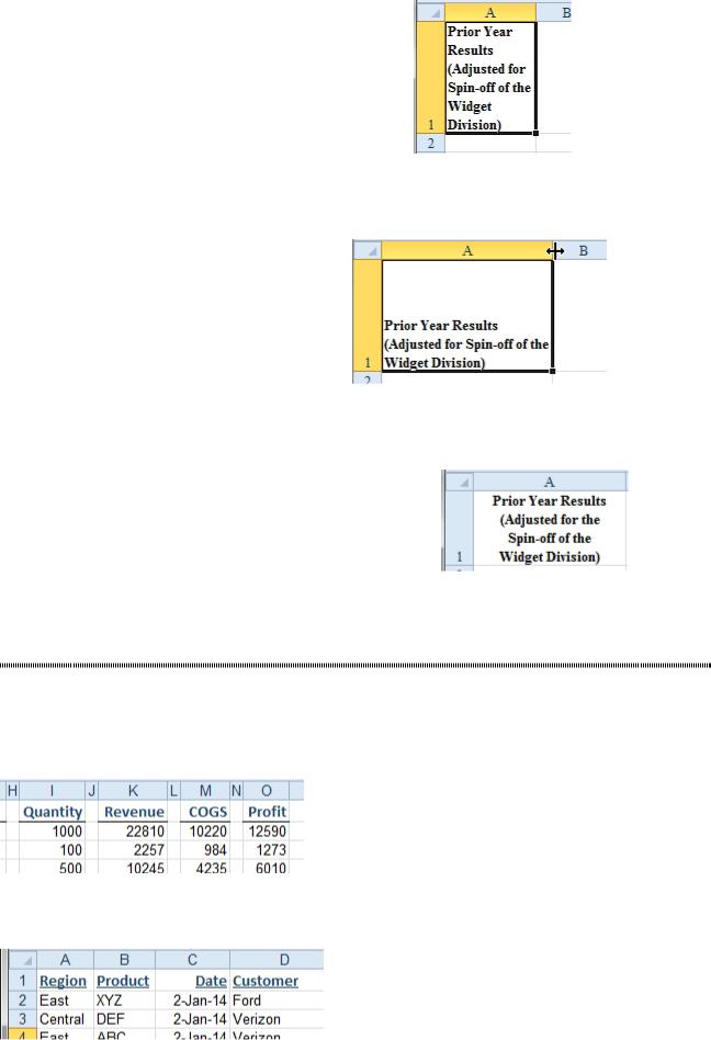
Turning on Wrap Text in this manner will probably work for a brief heading like “Prior Year.” However, if you want to have control over a long heading, such as “Prior Year Re- sults (Adjusted for Spin-off of the Widget Division),” then it is better to use Alt+Enter to specify exactly where the line break should occur. Wrap text uses a somewhat haphazard splitting of words.
Figure 580 Excel decides where to break lines.
As you make this column wider, Excel changes the way the words are wrapped. It is frustrating to keep adjusting the column widths until you get the words to wrap correctly.
Gotcha: After resizing a cell with Wrap Text, you often end up with a row height that is too tall. To correct this, you select the cell and then choose
Home, Format dropdown, Autofit Row Height.
Figure 581 Adjusting column widths to change line breaks rarely works.
Using Alt+Enter gives you absolute control over where the heading breaks. To create the figure below, type Prior Year Results <Alt+Enter> (Adjusted for the <Alt+Enter> Spin-off of the <Alt+Enter> Widget Division). You can make the column wider and center it for the perfect-looking cell.
Figure 582 Press Alt+Enter to wrap the text at logical points.
NO TINY BLANK COLUMNS BETWEEN COLUMNS
Problem: My Manager wants tiny blank columns between the columns.
Strategy: Plan on restating your numbers to the Securities and Exchange Commission. Tiny blank col- umns are a recipe for disaster. Someone will sort part of the data and not all of the data.
Most managers who demand this are doing it to make the bottom border under the headings look better.
Figure 583 Tiny blank columns are dangerous.
The manager here is using a bottom border to create the lines under the headings. He ends up using the bottom border because underlines just don’t look right. They only extend as long as the heading.
Figure 584 Underlines rarely make the manager happy.
PART 3: WRANGLING DATA |
235 |
|
|
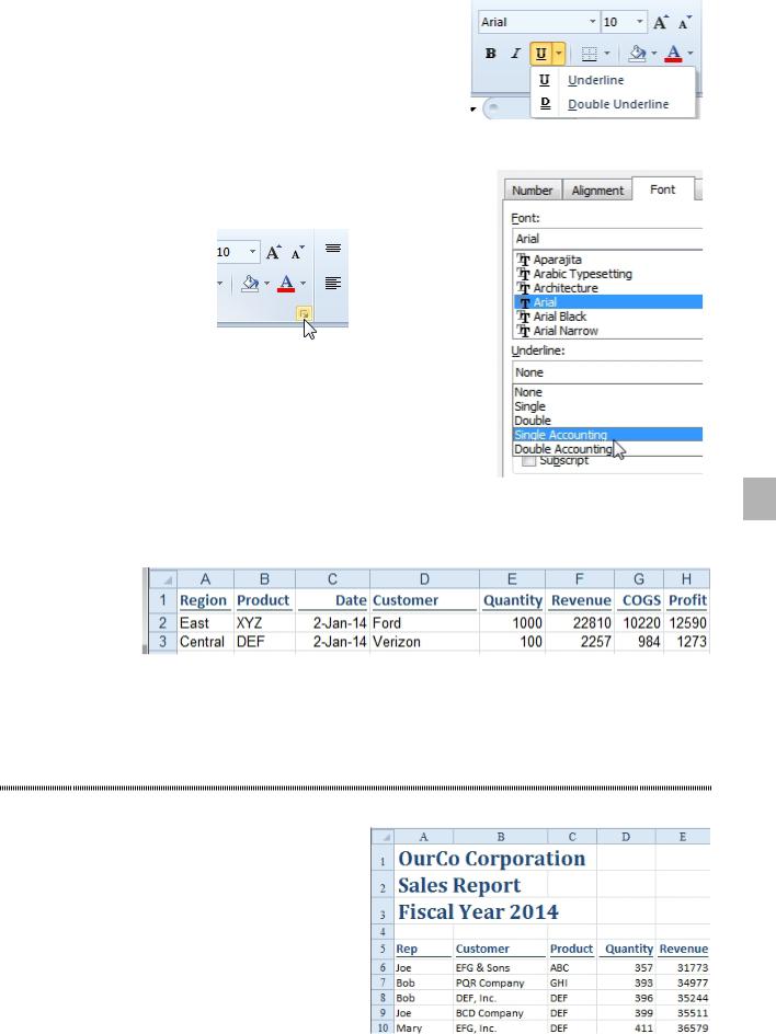
There is a solution that will make the manager happy. It won’t be found in the ribbon. Remember that the options in the ribbon are there to make Excel novices happy. If you are reading this book, you frequently have to go beyond the ribbon. In the ribbon, they offer two types of underlines.
Skip the ribbon choices. Instead, click on the dia- log launcher at the bottom of the Font group of the
Home tab of the ribbon.
Figure 586 Click the dialog launcher.
The underline dropdown in the Format Cells dialog offers four choices instead of two. Choose Single Ac- counting underline.
Figure 585 Two underline types in the ribbon.
Figure 587 The good choices are not in the ribbon. |
3 |
|
The result are bottom underlines that extend almost all the way across the cell, but not quite all the way. When printed, this will give the same look as back in Figure 583.
Figure 588 These underlines appear similar to gaps between columns.
Alternate Strategy: If your manager still demands the blank columns, you can put a word, such as
“blank” in the headings of the blank columns. Change the font color to white to no one sees those headings when printed. This will allow the entire data set to be treated as a contiguous set of columns.
HOW TO SORT DATA
Problem: I have sales data in a worksheet. I would like to sort the data by product within customer.
Figure 589 Sort by product within customer.
236 |
POWER EXCEL WITH MR EXCEL |
|
|
Strategy: Here’s what you do:
1. Select one cell within your data. The one cell can be in the heading row or any data row. Select Data, Sort. Whereas Excel 2003 only allowed sorting by three fields, Excel now offers up to 64 sort levels. Rather than the old dialog with the three fields, you now start with one field and add levels as neces- sary.
2. Choose Sort By dropdown, Customer.
3. Click the Add Level button. A new row will appear in the Sort dialog. Choose Then By dropdown,
Product.
Figure 590 Build as many sort levels as necessary.
4. Leave the Sort On and Order dropdowns at their default values. If, for some reason, you wanted the customers sorted in descending alphabetical order, you could change A to Z to Z to A. That might make more sense if you were sorting by revenue, but it is not likely that you need the customers sorted in reverse alphabetical sequence. If your data is set up correctly as outlined in ”How to Set up Your Data for Easy Sorting and Subtotals,” Excel will properly guess that your list has a header row.
5. Click OK to sort. Because Customer was the first sort key, all the records for “ABC Company” will sort to the top. Records for “ABC GMbH” will appear next.
Figure 591 The data is sorted.
Additional Details: When there is a tie—for example, the four records for “ABC GMbH”—those records will be sorted in ascending order by the product field. For instance, the ABC product record appears before the DEF product field. If there is still a tie, the records will remain in their original sequence from before the sort.
Alternate Strategy: If your data is properly set up in list format, you can select a single cell in the data and then use the AZ or ZA buttons on the
Data tab.
Note that these same icons are also in the Sort & Filter dropdown on the Home tab. If you don’t want the extra click of opening the dropdown or going to the Data tab, you can add the icons to the Quick
Access Toolbar.
If you use either method, Excel will sort the data by the column in which the cell pointer is currently located. Because Excel resolves ties by leaving the previous sequence in place, you can sort by product within customer. First, you select a cell in the Product field and click AZ to sort by product. Next, you select a cell in the Customer field and click AZ to sort by customer. The data will be sorted by customer, with ties sorted by product.
You can click the ZA button to sort in descending order.