


PART 3: WRANGLING DATA |
|
285 |
|
|
|
|
|
|
ADD A GROUP NUMBER TO EACH SET OF RECORDS |
||
|
THAT HAS A UNIQUE CUSTOMER NUMBER |
|
|
Problem: I have a list of invoice data. I want to number the records in such a way that the invoices for the first customer all have a group number 1 and the invoices for the next customer all have a group number 2.
Strategy: You can do this by sorting the data by customer. You need to add a new column A, with the heading Group. In cell A2, you enter the number 1 for Group 1. In cell A3, you enter the following formula, which will be used for the rest of the records:
=IF(C3=C2,A2,1+A2)
In plain language, this formula says, “If the customer on this row equals the row above, then use the group number on the row above. Otherwise, add 1 to the group number above.” You need to copy this formula down to all the other rows.
Figure 729 Assign each customer a group number. |
3 |
Results: Each record will be assigned a group number. Each customer will have a unique group number. |
|
|
|
In order to allow future sorting, you copy the formulas in column A and use Home, Paste dropdown, Paste |
|
Values to convert the formulas to numbers. |
|
DEAL WITH DATA IN WHICH EACH RECORD TAKES FIVE PHYSICAL ROWS
Problem: Sometime, back in the days of COBOL, a programmer was dealing with the constraints of the physical width of a page. The programmer built a report in which each record actually took up five lines of the report. I want to be able to analyze this data in Excel.
Figure 730 Transform this frustrating data set.

286 |
POWER EXCEL WITH MR EXCEL |
|
|
Strategy: Your goal is to get the data back into one row per record. This process involves adding two new columns, Group and Sequence:
1. Add a new row 1. Insert two new columns, A and B. Add the headings Group, Seq, and Text in A1:C1.
Figure 731 Add two new columns.
2. In column A, assign a group number to each logical record. One way to do this is to check to see if the first four characters of column C are ACCT. If they are, add 1 to the group number. In A2, enter the number 1. In A3, enter the formula =IF(LEFT(C3,4)=”ACCT”,1+A2,A2). (This is similar to the formula from “Add a Group Number to Each Set of Records That Has a Unique Customer Number”.)
Copy it down to all the rows. Excel will assign a group number to each logical group of records.
Figure 732 Use the IF function.
3. Design a formula for a sequence number. To do this, in cell B2, enter the formula =IF(A2=A1,B1+1,1). (This formula is like the one from “Number Each Record for a Customer, Starting at 1 for a New Customer”) Copy this down. This formula will number each record in the group. It should ensure that all the account numbers are on a Sequence 1 record.
Figure 733 Formula for sequence number.
4. (This step is critical.) Copy the formulas in columns A and B and paste them back, using Home,
Paste dropdown, Paste Values to ensure that you can safely sort the data.
5. Sort the data by the sequence number in column B. Your data will look like this.

PART 3: WRANGLING DATA |
287 |
|
|
|
Figure 734 Sort the data into record types. |
|
You have now managed to intelligently segregate the data so that all similar records are together. The |
|
|
contiguous range C2:C7 contains all the first rows from each record. Each of the line 1 records has three |
|
|
fields that really should be parsed into three separate columns. You can easily do this parsing with the |
|
|
Text to Columns Wizard. |
|
|
6. |
Select cells C2:C7. Select Data, Text to Columns to open the Convert Text to Columns Wizard. Select |
|
7. |
Fixed Width. Click Next. |
|
Excel should properly guess where your columns are. Click Next. |
|
|
8. |
Choose the heading for each column and define a data format. You don’t really need the word ACCT |
|
|
each time, so choose to skip the first, third, and fifth fields. Make the sixth field a date. When your |
|
|
|
|
|
information looks as shown below, click Finish. You will have data in three columns of Group 1. |
3 |
|
|
|
Figure 735 In Step 3, skip columns 1, 3, and 5. Choose Date for col. 6.
9. Change the heading in C1 to Acct, the heading in D1 to Inv, and the heading in E1 to Date. 10.Select and cut A8:C13 and paste into F2.
11.Delete Group & Seq from F & G.
12.Add the heading of Inv $ to F1.

288 |
POWER EXCEL WITH MR EXCEL |
|
|
13.Select F2:F6 and choose Data, Text to Col- umns. In Step 1 of the wizard, select Fixed Width and click Next. In Step 2 of the wiz- ard, Excel offers to split your data into three fields. There is no need to have one column for the word Invoice and another column for the word Total.
Figure 736 Excel suggests an extra column.
14.Double-click the line between Invoice and Total to delete it.
Figure 737 Double-click the extra line to delete it.
15.In Step 3 of the wizard, choose to skip the field that contains Invoice Total. Click Fin- ish.
Figure 738 Skip the field label.
16.Records for Groups 3 through 5 only have a single field without a heading. Copy C14:C19 to G2. Add a heading of Company.
17.Copy Group 4’s column C cells to H2. Add a heading of Address.
18.Copy Group 5’s column C cells to I2. Add a heading of City ST Zip.
19.Because the Group 6 records have no data—they are just dashed lines—delete these rows.
You now have all the fields, one line per record. 20.Delete the columns extra columns A& B.
Results: You now have a sortable, filterable, and reportable version of the original data set. Each record consists of one row in Excel.
Figure 739 You can now sort and analyze this data.
ADD A CUSTOMER NUMBER TO EACH DETAIL RECORD
Problem: I’ve imported a data set where the customer information appears once in column A, followed by any number of invoice detail records. At the end of the first customer, the next customer number is in column A and then there are detail records for that customer. You can not sort this data. The customer information needs to be in its own columns on each record.
PART 3: WRANGLING DATA |
289 |
|
|
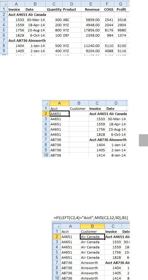
Figure 740 Another annoying report format.
Strategy: This is a common data format, but it is horrible in Excel. Here’s how you fix the problem:
1. Insert new columns A and B. Add the headings Acct and Customer. Here is the basic logic of what you want to do: Look at the first four characters of column C. If they are equal to Acct, then you know this row has customer information, so you take data from that cell and move it to column A. If the first four characters are anything other than Acct, you use the same account information from the previous row’s column A.
2. Enter the following formula into cell A2: =IF(LE
FT(C2,4)=”Acct”,MID(C2,6,5),A1). Copy this formula down through column A. you copy this formula down, it does the job. In cell A2, the IF condition is true and data is extracted from C2. In cell A3, the condition is not true, so the value from A2 is used. In cell A7, a new customer number is found, so the data from C7 is used in
A7. Cells A8 through A59 get the customer num- 3 ber from A7.
Figure 741 Use IF to extract and copy account number information.
Similar logic is needed in column B. In this case, though, you need to grab the customer name. You know that the word Acct and the space that follows it take up 5 characters. You know that your account number is another 5 characters, and then there is a space before the customer name. You therefore want to ignore the first 11 characters of cell C2. You can use the formula =MID(C2,12,50) to skip the first 11 characters and return the next 50 characters of the customer name. Use this formula as the TRUE portion of the IF function.
3. Enter the following formula into cell B2: =IF(LEFT(C2,4)=”Acct”,MID(C2,12,50),B1). Copy this for- mula down through column B.
Figure 742 Extract customer information.
You have now successfully filled in the account and customer. You need to change these formulas to values.