

PART 2: CALCULATING WITH EXCEL |
83 |
|
|
Strategy: It would be easier to understand the results if each component of every formula were named for what it represented and not just for the cell it came from. You can therefore use named ranges to make formulas easier to understand:
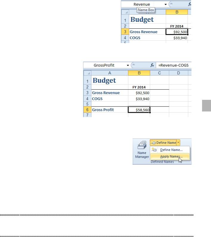
1. Select cell B3. In the Name box (the area to the left of the formula bar), type Revenue and press Enter.
2. Select cell B4. Click in the Name box, type COGS, and press Enter.
3. Clear the formula in B6. Reenter the formula and use the mouse to select the cells. Type =. Using the mouse, touch B3. Type -. Using the mouse, touch B4. Excel will enter the formula as =RevenueCOGS. This is easier to under- stand than a typical formula.
Gotcha: You need a lot of foresight to use this technique. In order to have this work automatically, you are supposed to be smart enough to create the range names before you enter the formula.
Figure 188 Type a name in the Name Box and press Enter.
2
Figure 189 This formula is easier to understand.
However, most people create a formula first and then de- cide to make the worksheet easier to understand. To assign range names after creating formulas, follow these steps:
1. Select Formulas, Define Name dropdown, Apply Names. Gotcha: Don’t click on the words Define
Name; click on the dropdown icon to the right of De- fine Name.
2. Select all the names you want to apply and click OK.
Figure 190 Apply Names is hidden in the
Define Name dropdown.
Results: A formula like =B6-B11 will be updated to =GrossProfit-Expenses.
Additional Details: One advantage of named ranges: they are always treated as an absolute reference.
You don’t need to add dollar signs to have the formula always point to that cell.
SEE ALL NAMED RANGES AT 39% ZOOM
Set your zoom to 39% or less. Excel outlines and labels each named range.
USE NAMED CONSTANTS TO STORE NUMBERS
Problem: I’ve seen how to assign a name to a cell. Is it also possible to assign a name to a constant? That could be useful for a number, such as a local sales tax rate, that changes periodically.
Strategy: Yes, you can assign names to constants. To do so, you follow these steps: 1. Select Formula, Define Name.
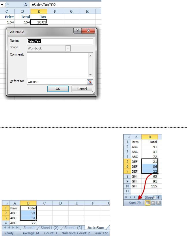
2. In the New Name dialog, type a name such as SalesTax in the Name text box. In the Refers To box, type 0.065 and then click OK.
3. In this workbook, you can now use a formula such as =SalesTax*D2.
84 |
POWER EXCEL WITH MR EXCEL |
|
|
Figure 191 A defined name holds 6.5%.
4. If the tax rate changes later, select Formulas, Name Manager. In the Name Manager, select the constant’s name and click Edit.
TOTAL WITHOUT USING A FORMULA
Problem: My manager called on the telephone, asking for the total sales of a particular product. I need to quickly find a total. Is there a faster way than entering a formula?
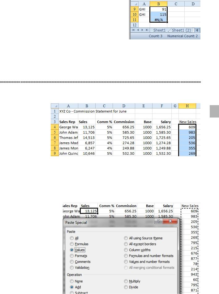
Strategy: While you’re on the phone with your manager, you can highlight the numbers in question. The QuickSum indicator in the status bar will show the total of the highlighted cells.
Additional Details: The status bar can simultaneously show a count, a numeric count, a sum, and so on. Right-click the status bar and choose the statistics you would like to show.
Gotcha: The Average, Numerical Count, and Sum parts of the sta- tus bar will ignore text entries within the selection. Below, Sum and Numerical Count only factor in B2:B3.
Figure 193 Select numeric cells, and the total appears in the status bar.
Figure 192 Count, Numerical Count, and Sum will ignore text cells.
If one of the highlighted cells is an error such as #N/A, the Sum and Average statistics will not appear in the status bar.
PART 2: CALCULATING WITH EXCEL |
85 |
|
|
Figure 194 An error cell will cause the Sum statistic to disappear.
Sometimes, when you are trying to find a lone #N/A within a column, it is fastest to start at the top of the column, hold down the Shift key, and start pressing PgDn. As soon as the Sum statistic disappears, you know that you have recently paged past the first #N/A error. (With 1 million rows, it might be faster to use Home, Find & Select, Go To Special, Errors.)
ADD OR MULTIPLY TWO COLUMNS WITHOUT USING FORMULAS
Problem: I’ve prepared a summary of sales by rep for the month. Due to an accounting glitch, someone gave me a similar file with additional sales made on the last day of the month. I need to add the new sales to the old sales. There is no need to keep the original two columns of partial month’s sales.
2
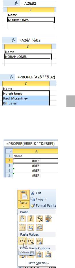
Figure 195 Add column H to column B.
Strategy: You can copy the new values in column H and use Home, Paste dropdown, Paste Special, Add to add the values to column B. Follow these steps:
1. Select H4:H22. Type Ctrl+C to copy the cells to the Clipboard.
2. Move the cell pointer to B4. Select Home, Paste dropdown, Paste Special. (Don’t select the large Paste icon; instead, choose the dropdown below the icon.)
3. In the Paste Special dialog box, choose the Add option in the Operation section. Optionally, also choose Values in the Paste section in order to preserve the formatting in column B. Click OK.
Figure 196 Choose Values and Add.

86 |
POWER EXCEL WITH MR EXCEL |
|
|
Results: The new sales values from column H are added to the values in column B. You can safely delete column H.
Gotcha: If column B is properly formatted and the tem- porary data in H is not formatted, the default Paste All option will cause the formats in column B to be lost if you choose only Add and not Values.
Additional Details: The technique described here for se- lecting Add in the Paste Special dialog has an interesting effect if you add cells to a range that contains a formula. Amazingly, Excel handles it correctly. For example cell D4 contains a formula.
If you select Add in the Paste Special dialog to add a val- ue to this formula, Excel changes the formula to add the value.
Additional Details: You can use the Operation section of Paste Special to handle other situations. In this figure, you might want to increase the contract rates by 2%. Type
102% in a blank cell. Copy that cell. Select the range of contract rates and use Paste Special, Values, Multiply.
This method was also used in Learn Excel Podcast episode
1348. Someone had received a dataset where a column of numbers needed to be divided by 100. For whatever reason, the creator of the data had put 123 instead of 1.23. The solution was to put 0.01 in a cell, copy the cell, then
Paste Special Multiply.
Figure 197 Excel adds the range on the Clipboard to column B.
Figure 198 Before pasting, this cell contains a formula.
Figure 199 After Paste Special Add, Excel modifies the formula.
Figure 200 Multiply this range by the 102% on the clipboard.
TYPE 123 TO ENTER 1.23
Excel can automatically insert s decimal point like the old adding machines. Go to File, Options, Advanced.
Figure 201 When you type 123, Excel will enter 1.23
JOIN TWO TEXT COLUMNS
Problem: I have data with first names in column A and last names in column B. I want to merge these two columns into one column.
Figure 202 You want to join A2 and B2 into a single cell.
PART 2: CALCULATING WITH EXCEL |
87 |
|
|
Strategy: You can use the ampersand (&) as a concatena- tion operator in a formula in column C. You change the formulas in column C to values before deleting columns A and B. These are the steps:
1. In cell C2, enter the formula =A2&B2.
Figure 203 Use & to join text.
2.To insert a space between the first name and the last name, join cell A2, a space in quotes, and cell B2, us- ing the formula =A2&“ ”&B2.
3.Copy the formula down to all the cells in the range.
2
Figure 207 Convert formulas to values.