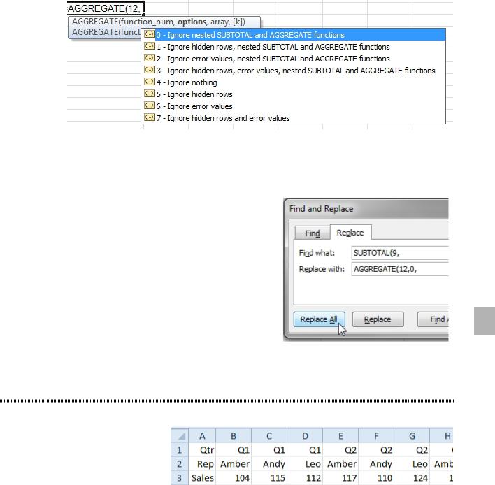
Figure 676 More options for what to ignore.

The AGGREGATE function offers potential for some incredible calculations. The new calculation arguments of 12 through 19 allow for array formulas, which would lead to some good additions for the Excel Gurus Gone Wild book. But to solve the median problem, it requires a simple Find and Replace.

To use a MEDIAN in a subtotal, you can use the Subtotal com- mand to sum the column in question.

Select the column. Use Find and Replace. Find SUBTOTAL(9, and replace with AGGREGATE(12,0,.

3

Figure 677 Change subtotals to medians.

HORIZONTAL SUBTOTALS

Problem: Why doesn’t Excel offer horizontal subtotals?

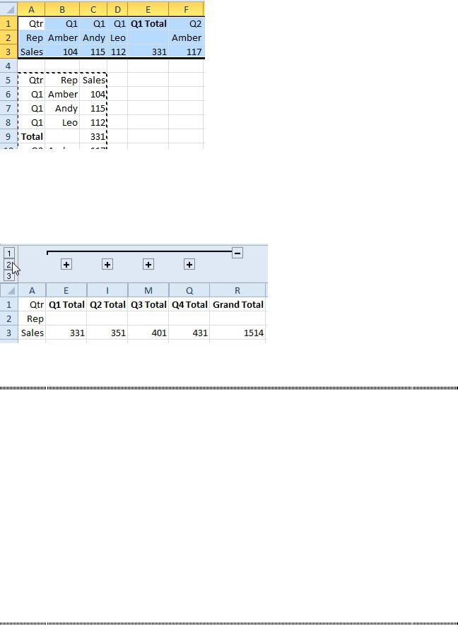
Figure 678 Add a subtotal in E for Q1.

Strategy: This is a great question. In my podcast episode 1001, I had several people write in to say that they regularly used this method to add horizontal subtotals. Although it is a lot of steps, if you use shortcut keys, it is actually fast.

1. Select the original data with Ctrl+*

2. Go a few rows below the data. Paste with Alt+E+S+E+Enter. 3. Alt+D+B to display the Subtotals dialog. Click OK.

4. Ctrl+C to copy the vertical data set with the subtotals. 5. Select cell A1.

6. Paste Transpose with Alt+E+S+E+Enter.

7. Fix the column widths with Alt+O+C+A.

Figure 679 Horizontal subtotals.

8. Delete the temporary table at the bottom.

9. Optionally, select columns B:D and choose Data, Group.

10.Select columns F:H and press F4 to re-do the group command.

11.Repeat step 10 for J:L and N:P.

12.Select B:Q and choose Data, Group.

You now have collapsible horizontal subtotals.

Figure 680 After manually adding groups.

BE WARY

Problem: By using the tips in this book, I have found myself processing data faster than ever before.

However, I’ve also begun to mess up data faster than ever before.

Strategy: It’s important to save and save often. It’s also a good idea to frequently check your data to make sure it’s reasonable. For example, if you work for a company with $100 million in annual sales, a quarterly sales report should not show $200 billion in sales.

Try to figure out problems as soon as they happen. Excel is an incredibly logical program. Everything hap- pens for a reason. If you can figure out the reason, you will master it in no time. Every “Gotcha” in this book represents a problem that has stung me in the past.

In 30 years of spreadsheet work, I have had only a few times when I could not find a logical explanation for something. If you are truly stumped, describe your situation on a message board such as the one at

MrExcel­ .com. The odds are that someone else has seen the same problem and figured it out.

You need to be aware of your data processing steps and occasionally do a reasonableness test to make sure your data still looks right. You should also save frequently with different file names if you are doing something new that you are unsure of. This way, you can go back to the IncomeBeforeSubtotals.xls file if you think you have done something wrong.

SEND ERROR REPORTS

Problem: I keep getting a fatal error on a particular workbook.

Strategy: If Excel crashes and offers you the chance to report the problem, please do so: All you have to do is click Send Error Report. Millions of people are using Excel, and if everyone reports their errors, Mi- crosoft will get a good statistical picture of the errors.

Figure 683 No blanks, but the data is resequenced­.

Figure 682 Remove blank rows.

Strategy: If the sequence is not important, you can sort the entire data range. Excel will move all blank cells to the bottom of the sort range. Here’s how you do it:

1. Move the cell pointer to A1. While holding down the Shift key, press the End key and then the Home key. Excel will select the entire range of data in the spreadsheet.

2. Select Data, Sort. In the Sort dialog, indicate that your data does not have a header row by uncheck- ing the My Data Has Headers box. Click OK.

Figure 684 Uncheck the My Data Has Headers box.

Results: The blanks will be removed from the list.

Excel’s Sort feature will always move blanks cells to the end of the sort. Sorting a column with blanks is a quick way to remove the blanks from the data.

REMOVE BLANKS FROM A RANGE WHILE KEEPING THE ORIGINAL SEQUENCE

Problem: Someone has given me data pasted from Word. There are a number of blank cells in the list. I want to eliminate the blank rows, but I need to keep the data in the original sequence.

Strategy: The trick described in “Remove Blank Rows from a Range”—sorting data to move the blanks to the end—is effective, but it destroys the original sequence of the range. Before sorting, you can add a temporary column with the original sequence numbers so that the data can be sorted back. Follow these steps:

1. Insert a new row 1. Place the cell pointer in cell A1 and then select Home, Insert, Insert Sheet Rows.

Because you have only one cell selected, only one row will be inserted.

2. In A1, enter a heading such as Symbol. In cell B1, enter a heading such as Sequence. Apply the cell style Heading 4 by using the Cell Styles gallery on the Home tab.

3. In cell B2, enter the number 1. Select B2. Hold down the Ctrl key while you drag the fill handle to the last row that contains data. The series 1, 2, 3 will extend down to 129 in row 130. Gotcha: If you get a series of 1s instead of 1, 2, 3, then you did not hold down the Ctrl key. Open the Auto Fill Options icon in C131 and choose Fill Series.

Figure 685 Ctrl+drag the fill handle.

Note: If the Auto Fill Options icon is obscuring some other data, it is fairly difficult to dismiss. One method is to resize any column.

4. Next, sort the data based on column A by selecting a single cell in column A and pressing the AZ button on the Data tab.

5. Press the End key and then the Down Arrow key to ride the range down to the last cell in A that contains data. Delete the rows below this last cell by highlighting the row numbers, right-clicking, and choosing Delete. (These are the blank cells. It is important to delete the sequence numbers from B for the blank cells so that they do not sort back into the data in the next step.)

6. Move the cell pointer to any value in column B. Click the AZ button on the Data tab to sort the data into the original sequence, without the blanks.

3

Figure 686 Sort by B to return A to the original sequence.

7. Delete the temporary column B by selecting Home, Delete, Delete Sheet Columns.

8. Delete the temporary row 1 by moving the cell pointer to A1 and selecting Home, Delete, Delete Sheet Rows.

Results: The blanks will be removed from the list, and the list will retain the original sequence.

Alternate Strategy: The previous steps work particularly well when your data set has many columns and you need to delete based on one column. If you truly have a data set that has a single column, try this faster method:

1. Select the range of data.

2. Select Home, Find & Select, Go To Special and in the Go To Special dialog, select Blanks and click

OK.

3. Select Home, Delete, Delete Cells, select Shift Cells Up, and click OK.

Excel will delete all the blanks and move the lower cells up.

Alternate Strategy: You can solve this with the Filter. Follow these steps:

1. Add a heading.

2. Select the entire data set.

3. Select Data, Filter. Open the Filter dropdown for the heading. Uncheck Select All. Scroll all the way to the bottom to choose (Blanks).

4. Re-select the visible rows, excluding the heading. 5. Select Home, Delete, Delete Sheet Rows.

6. Select Clear from the Sort & Filter group on the Data ribbon tab.