

178 |
POWER EXCEL WITH MR EXCEL |
|
|
Instead, hold down Ctrl+Shift. While holding Ctrl and Shift, then press Enter. In the formula bar, Excel will add curly braces around the formula. The result is correct.
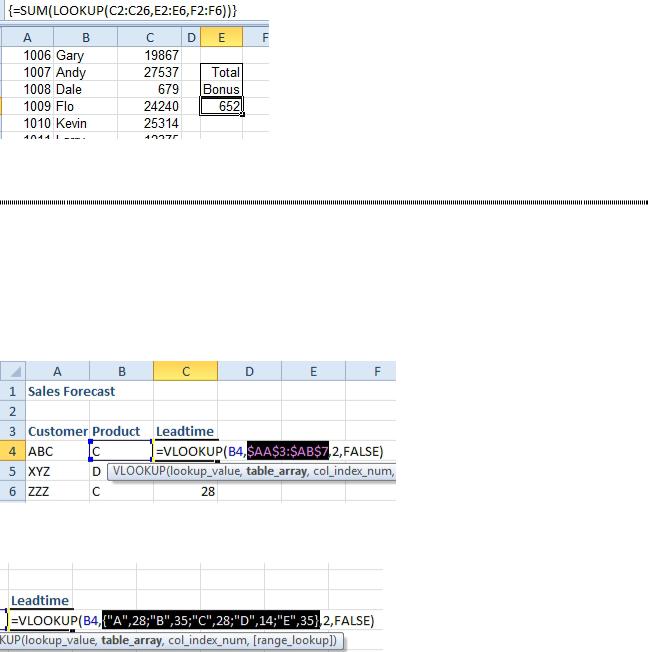
Figure 438 LOOKUP can return an array. VLOOKUP can not.
EMBED A SMALL LOOKUP TABLE IN FORMULA
Problem: I have a small 5-row lookup table hidden out in column AA:AB. The sales reps who use the spreadsheet might inadvertently delete a row in their data, deleting the lookup table. Can I put the lookup table somewhere that they won’t destroy it?
Strategy: One solution is to move the lookup table to a new worksheet and hide the worksheet. However, if the lookup table is small, you can embed it right in the VLOOKUP formula. Follow these steps:
1. Select the cell with the VLOOKUP formula.
2. Press F2 to put the cell in edit mode
3. Select the characters that represent the lookup table.
Figure 439 Select the table array portion of the formula.
4. Press F9. This calculates the selected portion of the formula. In this case, it puts {“A”,28;”B”,35;”C”, 28;”D”,14;”E”,35} into the formula.
Figure 440 Press F9. Excel inserts the array into the formula.
5. Enter the formula. Copy it down to the other rows. You can now safely delete the lookup table.
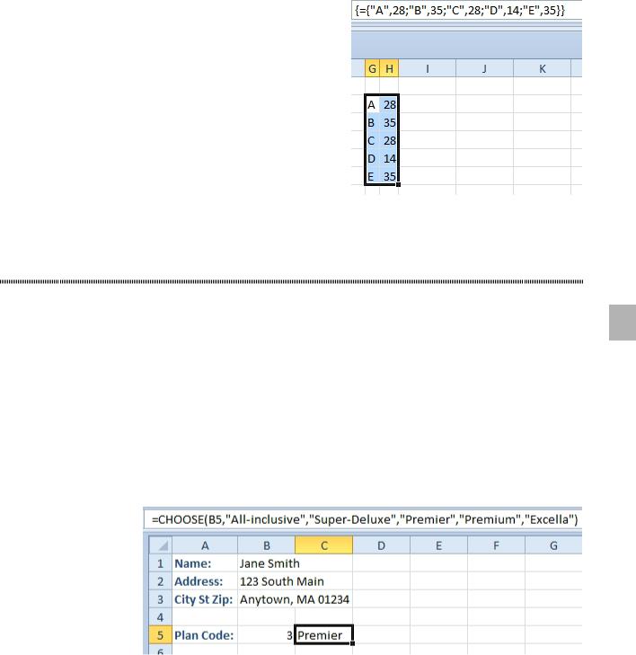
It helps to understand Excel’s array syntax. The curly braces indicate that this is an array. Each comma means you should move to a new column. Each semicolon means that you should move to a new row.
Gotcha: It is difficult to later edit the table. You can try to puzzle it out by staring at the commas and semi-colons in the formula bar. Or, you can copy the array and put it back in the worksheet. You have to follow these steps:
1. Select the array from the formula, including the curly braces.
2. Ctrl+C to copy the characters from the clipboard.
3. Select a five-row by 2 column blank section of the spreadsheet.
4. Type an equals sign. Press Ctrl+V. Press Ctrl+Shift+Enter. Excel will put the array back into the worksheet as an array formula. This looks OK, but you can not edit individual cells in the range.
PART 2: CALCULATING WITH EXCEL |
179 |
|
|
Figure 441 The table is back, but it is not editable, yet.
5. With the entire range selected, do a Copy and then Paste Values. You can now edit individual cells in the table.
I DON’T WANT TO USE A LOOKUP TABLE TO CHOOSE ONE OF FIVE CHOICES
Problem: I have to choose among five choices. I don’t want to nest a bunch of IF functions, and I really
don’t want to add a lookup table off to the side of my worksheet. Is there a function that will allow me to 2 specify the possible values in the function?
Strategy: In this situation, you can use the CHOOSE function.
The first argument of the CHOOSE function is a number from 1 to 254. You then specify the values for each possible number, entered as separate arguments. For example, =CHOOSE(2,”Red”,”Green”,”Blue”) would return Green.
It is a bit frustrating that you must specify each choice as a separate argument. I always want to specify a single range such as Z1:Z30 as the list of arguments but this will not work. However, if you already have the list of arguments somewhere, you don’t need to use CHOOSE; you can easily use VLOOKUP or INDEX in such a case.
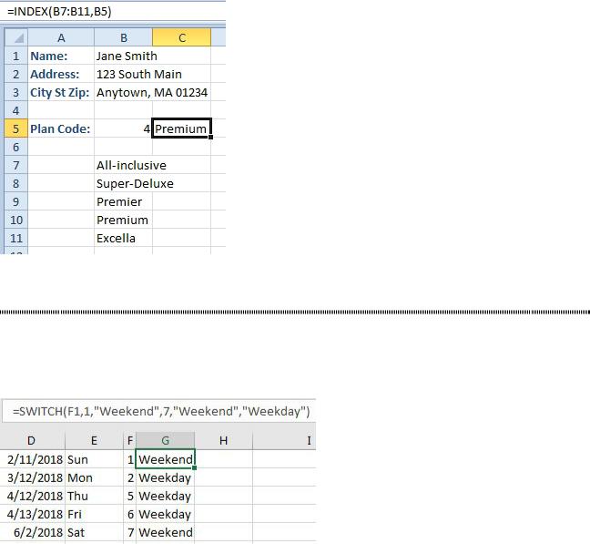
Here, a CHOOSE function returns the description of the plan number chosen in cell B5.
Figure 442 Choose is great for short lists.
Gotcha: CHOOSE works only if your plan codes are 1, 2, 3, and so on. If you have plan codes of A, B,
C, and so on, you should probably use a lookup table in an out-of-the way location. Or you could use
=CODE(B5)-64 to convert the A to a 1 and so on.
Additional Details: If you have a list of plan names somewhere, you might be tempted to enter
=CHOOSE(B5,B7,B8,B9,B10,B11). Instead, it is easier to use =INDEX(B7:B11,B5). The INDEX function will return the B5th item from the list in B7:B11.
180 |
POWER EXCEL WITH MR EXCEL |
|
|
Figure 443 Switch to INDEX if you have a list in a range.
IS THERE SOMETHING MORE FLEXIBLE THAN CHOOSE?
Problem: CHOOSE is strange in that it requires values such as 1, 2, 3. What if I need to check for values like 1, 7, 64?
Strategy: The February 2016 release of Office 365 adds a new function called SWITCH. Say that you want to return “Weekend” for values of 1 or 7, but “Weekday” for all other values.
Figure 444 The last argument in SWITCH is used for all other values.
SWITCH can also work with text. =SWITCH(J1,”Andy”,5,”Bill”,7,”Fred”,1,”Ralph”,3,99) can be used to assign 5 to Andy, 7 to Bill, 1 to Fred, 3 to Ralph and 99 to any other value.
PART 2: CALCULATING WITH EXCEL |
|
181 |
|
|
|
|
LOOKUP TWO VALUES |
|
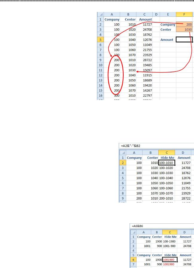
Problem: I have to lookup two values. I need to match both a company code and a cost center.
Figure 445 Match both the Company and Center. |
2 |
|
|
Strategy: There are three solutions to this problem: (a) Concatenated key, (b) OFFSET, or (c) SUMIFS.
The concatenated key will only work if you are allowed to add a new column to the left of column C. The
SUMIFS will only work if the value to be returned is numeric. The OFFSET will only work if all of the company codes are sorted together as shown above.
With a concatenated key, you will insert a new column before the Amounts in column C. You want to join column A, a unique separator, and column B. For example, =A2&”-”&B2 would produce a key of 100-1010.
Figure 446 Build a concatenated key in your data.
The separator text is optional. In real life, you might have two company/center combinations that would look the same once joined. Using a dash in between will prevent this ambiguity.
Figure 447 Using a dash prevents the identical key fields in red.
182 |
POWER EXCEL WITH MR EXCEL |
|
|
Once you have the concatenated key in the lookup table, you can join the key fields on-the-fly in your VLOOKUP formula:
=VLOOKUP(G2&”-”&G3,$C$2:$D$22,2,FALSE)
Figure 448 Join the two key fields as the first argument of VLOOKUP.
As mentioned earlier in this topic, this method only works if you are able to add the concatenated key to your data. It is fine to hide column C so no one see it, but you have to have the field there.
Alternate Strategy: If the value that you are trying to return is numeric, you can use DSUM or SUMIFS. For details, see "Calculate Based on Multiple Conditions" on page 157.
Figure 449 The new SUMIFS would solve the problem.
Alternate Strategy: Use the OFFSET function. Purists will argue that OFFSET is a volatile function and therefore slows down your calculation times. However, OFFSET will often solve problems where you need to reference a range that is moving or resizing.
OFFSET is used to point to a range. The location and size of the range is calculated as the formula is being calculated.
OFFSET allows five arguments. At least one of the four final arguments should be a formula that is cal- culated on the fly. When OFFSET is set up to return a range of cells, you will find yourself using OFFSET inside of another function such as SUM, or in this case, inside of VLOOKUP.
The syntax is =OFFSET(Reference,Rows Down from There, Columns Right from There, Rows Tall, Col- umns Tall). For example, you could start with a reference of B1, move down N rows, move right 0 rows, make the range be 7 rows tall and 2 columns wide.
In the next figure, a MATCH function in F5 figures out where the lookup table for this company begins. The COUNTIF in F6 figures out how tall the lookup table should be. Both of these numbers will feed into an OFFSET function that is shown for illustration in F7. The actual formula is found in F9, where the OFFSET is used to describe the lookup table in the VLOOKUP formula.