2.From the Design tab, select the Layouts gallery. It initially shows four other layouts besides the one you used. Click the bottom arrow to open the gallery.

Figure 1381 Click the More arrow to open the gallery.

3. Initially, the Layouts gallery shows only the layouts from the same category as your existing graphic. To choose from the complete set of layouts, choose the More Layouts option at the bottom.

Figure 1382 You see more layouts, but not all of them.

4. Choose the All category and then choose a new layout.

Results: Your existing message will be presented in a completely new SmartArt layout.

FORMAT SMARTART

Problem: SmartArt always starts out as a boring blue diagram. What formatting options are available?

Strategy: You can use two galleries on the Design tab of the ribbon to quickly add color and effects to a graphic: The Change Colors gallery and the SmartArt Styles gallery.

The Change Colors dropdown offers more than three dozen color styles. The Colorful row offers five combi- nations of the six accent colors in the current theme. The Primary Theme Colors offer two light style and one dark basic style. The remaining six rows offer variations on each of the six accent colors.

Figure 1384 Add color to SmartArt by using the Colorful row choices.

Gotcha: Each of the accent rows offer Outline, Colored Fill, Gradient Range, Gradient Loop, and Trans- parent Gradient Range columns. Of these five columns, only the first two seem to make any sense. For example, see the figure below. It shows five horizontal SmartArt graphics. Each row is formatted with a different accent color scheme. The Outline and Fill graphics look okay. In the third row, the Gradient

Range graphic goes from dark to light, making it appear as if the company will be fading away by the final shape. In the fourth row, the Gradient Loop graphic is worse. Shapes alternate from dark to medium to light to medium to dark. This makes me think that somehow the 2014 and 2016 shapes are supposed to be related. In the fifth row, the Transparent Gradient Range graphic suffers the same problem as in row 3.

Figure 1385 Only Outline and Colored Fill graphics look okay.

Additional Details: You can easily add effects by choosing one of the 14 styles from the SmartArt Styles gallery. The first five styles are 2-D styles and labeled as “Best Match for Document.” The remaining nine styles are 3-D styles.

Figure 1386 The first few 3-D styles create nice effects.

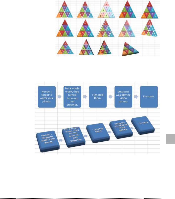
The 14 graphics below demonstrate the styles available. I use the second 3-D style most of the time. It creates a nice effect but is still readable.

Figure 1387 Examples of the 14 layouts.

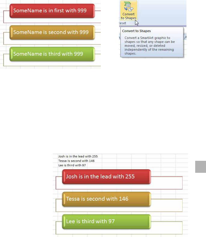
Gotcha: If you move far into the 3-D styles, many of them are unreadable. Perhaps Microsoft is doing us a favor. For example, perhaps the ninth style, known as Birds Eye Scene, is designed for messages in which you need to deliver bad news. You can say that you showed the information, but no one will really be able to read it. This figure shows the original message and the message rendered in Birds Eye Scene.

4

Figure 1388 Apply a little Birds Eye Scene to bad news.

Additional Details: If you change the theme on the Page Layout tab, you will have new colors available in the Colorful row, but you will also inherit new effects that change the options available in the Smart- Art Styles gallery. If you only want new colors, you can use the Colors dropdown on the Page Layout tab instead.

Additional Details: If you are using a layout that includes picture placeholders, click the placeholder to browse for a photo.

SWITCH TO THE FORMAT TAB TO FORMAT INDIVIDUAL SHAPES

Problem: Birds Eye Scene style notwithstanding, (see Figure 1388 above), I’ve found that most SmartArt formatted using the Design ribbon looks good. Fonts remain consistent throughout. Shapes have similar effects. While giving Microsoft control over font size will usually create a suitable graphic, sometimes I need to tweak the font used within one shape.

Strategy: All the tools on the Format tab of the ribbon will allow you to change elements of a SmartArt graphic.

To change elements of a SmartArt graphic, select a single shape in your graphic. The Shapes group will allow you to change the shape or size of the individual shape.

Figure 1389 Tweak size or shape of one element of a SmartArt graphic.

With a single shape selected, you can use any of the tools in the Shape Styles group to change the shape formatting. You can use any of the tools in the WordArt Styles gallery to add effects to the text. You can use any of the formatting tools in the Home tab of the ribbon to change font or size.

Gotcha: When you change shapes on the Format tab, Microsoft will often quit updating font sizes in re- sponse to text changes. You should get your graphic as close to finished using the Design tab before moving to the Format tab.

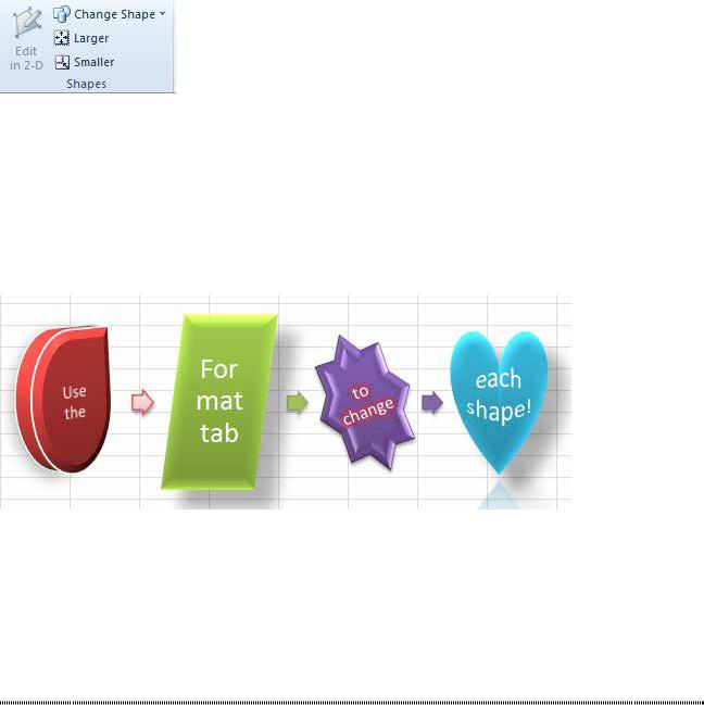
Additional Details: If you find yourself making many changes on the Format tab, you will lose the con- tinuity of the graphic. The graphic below shows some of the many changes possible with the Format tab.

Figure 1390 If you are not careful with the Format tab, chaos results.

In this figure, each shape was changed using the Change Shape menu. The second shape was made larger, and the font size was increased on the Home tab. The Text Effects glow setting was used to apply a glow to text in the third shape. The green rotation handle was used to rotate the third shape. WordArt Styles, Text Effects, Transform was used on the text in the fourth shape, and Shape Styles, Shape Effects, Reflec- tion was used to add a reflection. In the first shape, a preset from the Shape Effects dropdown was used.

Although it is not recommended, you can use the Format tab to tweak many aspects of an individual shape.

USE CELL VALUES AS THE SOURCE FOR SMARTART CONTENT

Problem: As discussed in "Place Cell Contents in a Shape" on page 522, Excel has been able to use val- ues from an Excel cell as the source for text boxes on AutoShapes for fifteen years. It would be obvious to anyone that the best use of SmartArt would be to populate the text pane with cell references. However, nothing I try allows me to specify cell A1 as the source in the text pane. What’s going on?

Strategy: Amazingly, Microsoft did not hook up this feature in Excel! It was obvious to you, and it was obvious to me, but Microsoft didn’t think to include it.

From Microsoft’s point of view, SmartArt is primarily a PowerPoint feature that is also available in Word and Excel. Heck, in PowerPoint, Microsoft even made the Convert Any Text to SmartArt functionality. But because PowerPoint doesn’t offer cells and formulas, it was not a priority to enable this feature in Excel. Luckily, I have a workaround.

Follow these steps to build a SmartArt graphic that is tied to cell values:

1. Build a SmartArt graphic with the correct number of shapes. Type sample text of about the correct length in the shapes.

2. Choose a color scheme from the Design tab.

3. Choose a style from the Design tab. Get the diagram looking exactly as you will want it to appear, because after step 4, Excel will stop automatically formatting the SmartArt.