Problem: I have the data set shown below. I need live formulas that replicate this data set on another worksheet. When I set up the formulas, I get zeroes where the blank cells are located. I can use

=IF(ISBLANK(A1),””,A1) to suppress the zeroes, but then if I try to do any math on A1 in the worksheet copy, I am getting #VALUE errors.

Figure 383 Set up a link to replicate a table on another worksheet.

Figure 384 The result is showing zeroes instead of blank cells.

If you change the formula to display nothing, the zeroes go away, but there is another prob- lem. A formula such as =C2+B2 will display a #VALUE! error while it would have worked fine in the original data.

Strategy: Go back to the formula shown in

Figure 384. Use one of two methods to force

Excel to not display zero values.

Figure 385 The IF solves one problem, but creates another.

The first method is to suppress the display of zero for the entire worksheet. Go to File, Op- tions, Advanced. Scroll down to Display Options For This Worksheet. Uncheck the box for Show a Zero In Cells That Have a Zero Value.

Gotcha: this setting affects the entire worksheet. What if you want zeroes to appear in another range on this worksheet?

Figure 386 Zeroes don’t appear. The formula in F2 works as expected.

In that case, you can use a custom number format to suppress zeroes in a particular range. Select B2:E11. Press Ctrl+1 (Ctrl+One). On the Number tab, choose

Custom from the listbox on the left. Type a custom number format of 0;-0;. This code will display positive numbers and negative numbers, but suppress zero values.

Figure 387 Use 0;-0;.

COUNT RECORDS THAT MATCH A CRITERION

Problem: I have a large data set. I want to count the number of records that meet a certain criterion.

2

Figure 388 Count males and females.

Strategy: You use the COUNTIF function, which requires two arguments: a range of cells that you want to test and a criteria. To count the records where the gender is M, you use =COUNTIF(B5:B60,“M”).

Figure 389 COUNTIF function looks through a range, counting matches.

Note that the second argument, “M”, tells Excel to count records that are equal to M. Because this function is not case-sensitive, the function will count cells with values of M or m.

If you want to count the records where the age is a specific number, you can write the formula either with or without quotes around the number:

=COUNTIF(D5:D60,32)

=COUNTIF(D5:D60,“32”)

You can also establish a criterion to look for items that are below or above a certain number:

=COUNTIF(D5:D60,“<21”)

A criterion can include a wildcard character. To find any text that contains XYZ, you use the following formula:

=COUNTIF(A2:A999,”*XYZ*”)

Problem: I need to build a summary table using COUNTIF functions. How can I enter one formula that can be copied?

Strategy: Use a cell reference as the second argument in the COUNTIF function. Here’s how:

1. Set up a table below your data and place all the possible values for a column, such as department, in column A.

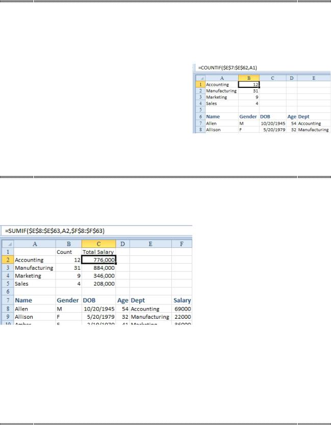
2. In column B of the first row, enter =COUNTIF($E$7:$E$62,A1). Note that you should press the F4 key after selecting E7:E62 to make the first range absolute. This will allow you to copy the formula to other rows.

3. Copy the formula down for the other departments.

Figure 390 Count of records by department.

SUM RECORDS THAT MATCH A CRITERION

Problem: That COUNTIF function is cool. Is there a way to sum all records that match a criterion?

Strategy: There is a SUMIF function that works similar to COUNTIF. In this case, you would look at all values in E8:E63 to see if they are equal to “Accounting”. If they are, you want to add up the corresponding value from F8:F63.

Figure 391 Sum values from F if E is the right department.

The one difference from COUNTIF is that the SUMIF function usually requires you to specify the sum range as the third argument. (I say usually, because you might sometimes want to add up all salaries over $60000. In that case, the first and third arguments would both be F8:F63, so you can omit the third argu- ment).

Additional Details: Starting in Excel 2007, Microsoft added an AVERAGEIF function. This seems fairly redundant to me, since you could easily do =C2/B2 in the current example rather than doing an AVER- AGEIF formula.

CAN THE RESULTS OF A FORMULA BE USED IN SUMIF?

Problem: Can the results of a formula be used as the criteria? I would like to add all numbers that are above average.

Strategy: The second parameter of the SUMIF/COUNTIF can be a calculation, but you must concatenate a comparison operator in quotes with the formula. Consider this formula:

=SUMIF($F$6:$F$61,”>”&AVERAGE($F$6:$F$61),$F$6:$F$61)

The criteria is “>”&AVERAGE(F6:F61). Excel first calculates the average, then joins the operator with the result. In the second step of evaluating the formula, Excel has changed the formula to “>39535.71”.

Figure 392 The criterion is built from a formula.

CALCULATE BASED ON MULTIPLE CONDITIONS

Say that you want to calculate average salary by department and age range. This requires three sets of criteria. The department has to match. Since you want to report on ages by decade, you need to look for ages >=30 and <40.

Figure 393 Averaging based on three conditions.

Note: The data being averaged is similar to the data in the previous several topics. I am not showing col- umns A:F in the above figure because it would be too small. See Figure 388 for the columns in the data set.

The headings are in row 1 and the data is in rows 2 through 57.

The first argument is the range with the values that you want to average. This is F2:F57.