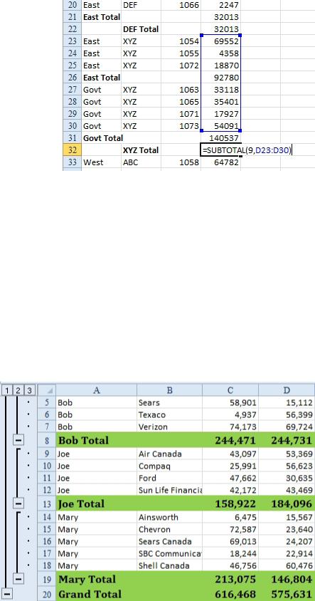
If you then total by region, you will have set up groups that make no sense. Note that the XYZ total in D32 includes both Govt and East records.

Figure 666 Chaos ensues.

Additional Details: In Excel 95, there was no workaround for this problem. In Excel 97, Microsoft added the rule that XYZ rows separated by a blank row would be handled correctly. Thus, you need to add sub- totals by region first.

Figure 667 Format only the subtotal rows.

Problem: My manager wants me to add a blank line between sections of a subtotal report.

Strategy: This is a fairly standard request. Quite simply, data looks better when it is formatted this way.

But there is no built-in way to do this with Excel. I’ve tried many methods. There are two methods that will work here. One method is simpler but is really cheating; you only make it look like you added a blank row. The second method is convoluted but about 50% easier than the method I described in the previous edition of this book.

The first method is to try to fool the manager by making the total rows double height, with the totals verti- cally aligned to the top. This method may work if you are printing the report to give to the manager. It will give the appearance that a blank row has been inserted. Here’s how you do it:

1. To do this easily, add subtotals, collapse to level 2, and select all subtotal rows from the first subtotal to the last subtotal.

2. Select Home, Find & Select, Go To Special, and from the Go To Special dialog, select Visible Cells Only and click OK. (You can use Alt+; as the shortcut for Visible Cells Only.)

3. Select Home, Format dropdown, Row Height. Depending on your font, the row height will probably be between 12 and 14. Say that the height is 12.75. Mentally multiply by 2 and type 25.5 as the new height.

4. In the Home tab of the ribbon, click the Align Top icon.

5. Choose the 3 Group & Outline button to display the detail rows again.

Although you can see that there is no blank row after the subtotals in rows 8 and 13, when you print the report for your manager, it will appear to have a blank row.

Figure 668 There is not a blank row between rows 8 and 9.

This method will not work if you have to send the data set to the manager via e-mail. The manager may be smart enough to want to stop at each subtotal by pressing the End key, and this will not work with the double-height rows.

Alternate Strategy: This method is far more complex than the one just described but creates the desired result. Follow these steps:

1. Add subtotals as described previously. Click the 2 Group & Outline button.

2. Insert a new temporary blank column A to the left of the current column A. To do this, select any cell in column A and then choose Home, Insert, Insert Sheet Columns.

3. Select the cells in column A from the first subtotal down to the last subtotal. 4. Use Alt+; to select only the visible rows.

9.Select Home, Insert, Insert Sheet Rows. Excel will insert 1 row above each row in your selection.

Through the combination of steps 7 and 8, you were able to make a selection that consisted of each cell underneath the subtotals. Inserting a new row above these cells creates the result.

Figure 670 Insert a row above each cell in the selection.

Results: You will have added the blank rows requested by the manager. You can now delete column A.

Gotcha: When the blank rows are in, you may have a difficult time getting rid of the subtotals. If you select cell A2 and choose Data, Subtotal, Remove All, Excel will delete only the first subtotal. In order to delete all the subtotals, you have to select the entire range before calling the Subtotal command. One fast way to do this is to click on the blank gray box above and to the left of cell A1. This box will select all cells in the worksheet. Now when you choose Data, Subtotal, you will find that Excel has selected all the subtotals.

Click Remove All to remove the subtotals.

SUBTOTAL ONE COLUMN AND COUNT ANOTHER COLUMN

3

Problem: I want to subtotal revenue and count the number of re- cords. The Subtotal dialog offers 11 different summary functions including two counting functions. How do I change the function for different columns? I’ve tried adding the SUM to Revenue, then do- ing subtotals a second time to count the customer, but the subtotals end up on two different rows.

Strategy: When you add subtotals, Excel makes use of a function called =SUBTOTAL(). The first argument of the SUBTOTAL func- tion tells Excel which summary function to use.

=SUBTOTAL(9, is the argument for sum. There are 11 functions to choose from. Microsoft arranged the arguments alphabetically.

Figure 671 SUM is 9th.

The solution is to add automatic subtotals to the numeric columns and the text column that you want to count. Of course, the totals on the text column will be zero.

Figure 672 Total a text column.