

100 |
POWER EXCEL WITH MR EXCEL |
|
|
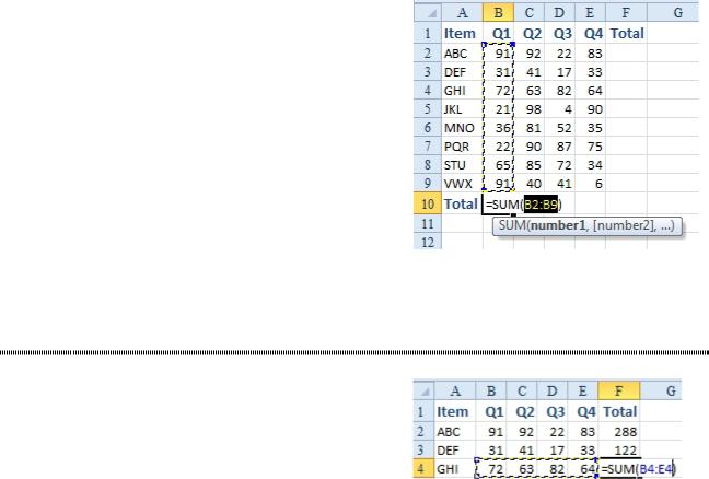
1.Place the cell pointer in cell B10. Click the AutoSum button. Excel analyzes your data and predicts that you want to total the range of numbers above the cell pointer. Excel proposes the provisional formula
=SUM(B2:B9).
2.Review the range in the proposed formula, if needed. If the range is correct, press Enter to accept the formula. Excel displays the total.
3.With the mouse, drag the fill handle (the square dot in the lower-right corner of the cell pointer) to the right to include cells C10 through F10 and then release the mouse button. The formula will be copied to all five columns.
Additional Details: You can use Alt+= instead of clicking
the AutoSum button. Figure 239 Excel proposes a formula.
Gotcha: Blank cells in the sum range will cause AutoSum to exclude cells above the blank cell.
AUTOSUM DOESN’T ALWAYS PREDICT MY DATA CORRECTLY
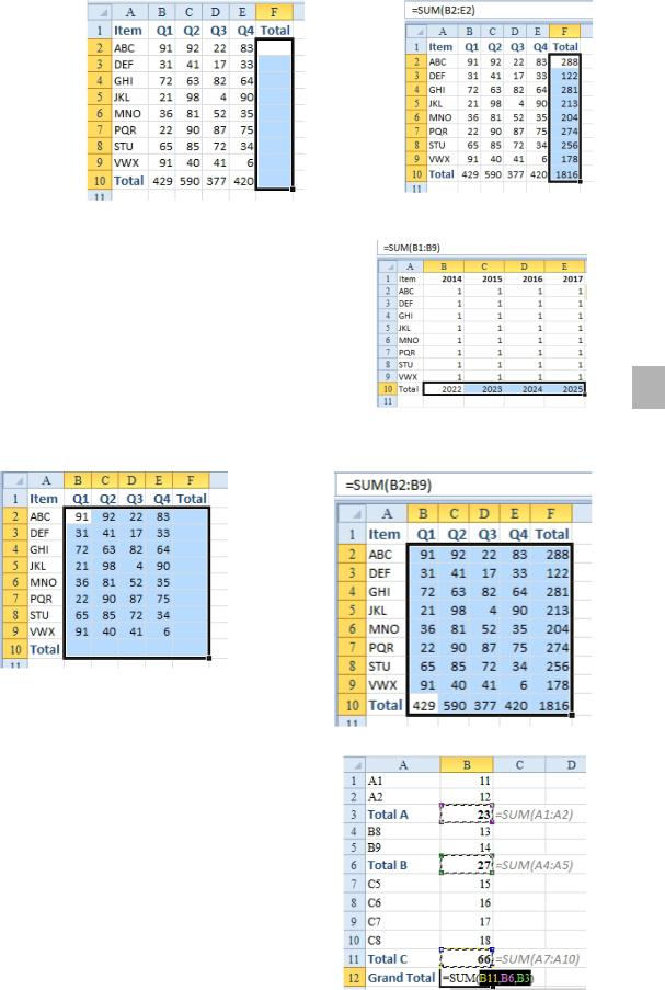
Problem: When I use the AutoSum button, Excel some- times predicts the wrong range of data to total. Below,
AutoSum worked fine in F2 and F3, but in cell F4, Excel thought I wanted to total the rows above F4. How do I enter the correct range?
Strategy: After you press the AutoSum button, the provi- sional range address is highlighted in the provisional for- mula. Using your mouse, you highlight the correct range.
Figure 240 Excel chose the column instead of the row
AutoSum will work correctly in F2 and F3. It will predict that you want to sum the data in that row. How- ever, in cell F4, Excel has a choice: either sum the two cells in that column or the four cells in the row. Excel always chooses to sum the two cells above in this situation.
After you press the AutoSum button, note that F2:F3 is highlighted in the formula. This allows you to enter the correct range. There are three methods:
●● With the mouse, highlight B4:E4 and press Enter. ●● With the keyboard, type B4:E4.
●● Using the arrow keys, press the Left Arrow key to move to E4. While holding down the Shift key, press the Left Arrow key three times to highlight B4:E4.
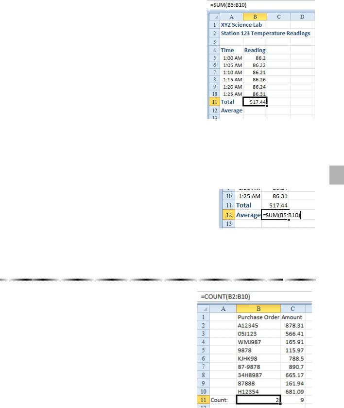
AutoSum can also fail when one number in your range contains a SUM formula. The provisional formula will offer to sum a formula extending up to but not including the previous SUM formula.
Alternate Strategy: You can choose to enter all the totals at one time by using the AutoSum button.
This is faster than the methods just described and will eliminate the problem described. Follow these steps:
1. Highlight the entire range that needs a SUM formula.
2. Press the AutoSum button. Excel makes a prediction and fills in the total formulas automatically.
Excel does not show the provisional formula, so check one formula to see that it is correct.
PART 2: CALCULATING WITH EXCEL |
101 |
|
|
Figure 241 Select the entire range
Gotcha: Headings that contain dates or numeric years can really cause problems for AutoSum. Excel will usually get fooled into including the heading in the sum. Be extra cau- tious when using AutoSum in these situations. Here, Excel incorrectly included the headings in row 1.
There is an amazing workaround. You can select the cells to be totaled plus one extra row and one extra column.
When you click the AutoSum button, Excel correctly adds SUM formulas in the total row and total column.
Figure 244 Select an extra row and an extra column
Another AutoSum oddity is shown here. The cell- pointer is directly below a SUM function. There are additional SUM functions in the range that would normally be included in the AutoSum. In that case, AutoSum will only include the other SUM functions.
Figure 242 Provisional formulas are not displayed.
2
Figure 243 The numeric year headings are mistakenly included.
Figure 245 Add totals in one click.
Figure 246 AutoSum only sums the SUM formulas.
102 |
POWER EXCEL WITH MR EXCEL |
|
|
|
USE THE AUTOSUM BUTTON TO ENTER AVERAGES, MIN, MAX, AND COUNT |
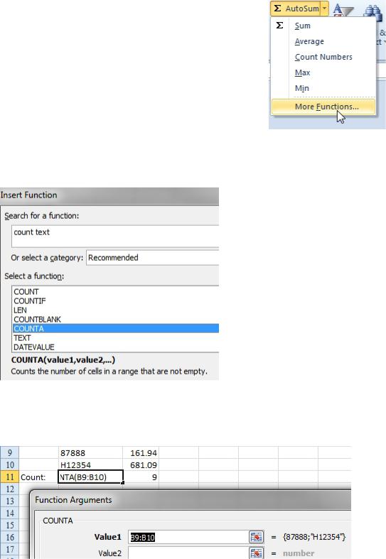
Problem: I often enter totals formulas, but in this case, I need to enter an average formula. How can I do it quickly?
Figure 247 Average the readings.
Strategy: You use the dropdown arrow located next to the AutoSum button. Instead of selecting Sum, you select the Average option.
Figure 248 The AutoSum dropdown offers additional functions.
DITTO THE FORMULA ABOVE
Problem: I routinely have to sum and average the same range. The sum is easy enough with the Auto-
Sum. But when I try to do the average, the formula above is in the way.
PART 2: CALCULATING WITH EXCEL |
103 |
|
|
Figure 249 Add a total and an average.
Strategy: Go to cell B12. Hold Ctrl while you press the key with the ditto mark. (Remember the ditto mark from elementary school? It was a double quotation mark: “.) Technically, you are pressing Ctrl+Apostrophe, but think of it as Ctrl+Ditto.
Excel will make an exact copy of the formula above and show you the provisional formula. Why is this bet-
ter than a copy and paste? A copied formula would change the B5:B10 range to be B6:B11. A dittoed range 2 will keep the reference to B5:B10.
Figure 250 Ctrl+Ditto copies the formula without changing the reference.
From the point in the figure above, you can press F2, Home, Right Arrow, AVERAGE, Delete, Delete,
Delete, Enter.
THE COUNT OPTION OF THE AUTOSUM DROPDOWN DOESN’T APPEAR TO WORK
Problem: I am using the Count option from the AutoSum dropdown on the toolbar, but it does not appear to provide consistent results. Cells B11 and C11 both contain counts of the cells in rows 2 through 10 of each column. One function indicates that there are nine entries; the other function indicates that there are only two. Clearly, both columns have nine entries. What is the problem?
Strategy: The COUNT function will count only numeric entries. If you need to count all entries, you have to use the COUNTA function. One solution is to edit the formula in B2 by adding an A after the T in COUNT. The other method is to enter the formula correctly in the first place. Here’s what you do:
Figure 251 Why does Excel think the count is two?
104 |
POWER EXCEL WITH MR EXCEL |
|
|
1.Put the cell pointer in B11. Select AutoSum drop- down, More Functions. There are hundreds of func- tions available, and it can be difficult to remember where a function is; for example, you don’t know if
COUNTA is in the Math & Trig section or somewhere else.
Figure 252 The AutoSum dropdown can lead to more functions.
2.In the Search for a Function box, type the words “count text” then click Go. Excel will propose pos- sible functions. You can click on each function to see a one-line description of what the function does.
Figure 253 Excel proposes functions related to your search.
3. Click on COUNTA and then click OK. Excel will analyze your data and predict the range that you want to use. However, Excel is not good at predicting data when the range contains numeric and alphanumeric entries. The Function Arguments dialog box appears. In this particular case, Excel assumes that you only want to use COUNTA on the range B9:B10.
Figure 254 Excel guessed the range incorrectly.
4. If you can see the data on the worksheet, use the mouse and highlight the correct range. If the range is behind the dialog, click the Reference icon at the right edge of the text box. Then highlight the correct range. Alternatively, you can drag the dialog box until your range is completely visible.
5. Click OK in the Function Arguments dialog to accept the formula.
Results: The COUNTA function returns the desired value.