CHAPTER 2

The architecture of modern graphics processors

Programmable graphics processors (GPUs) have emerged as a low-cost, high-performance solution for general-purpose computations. To understand the nature of the architecture of the graphics processors, it is necessary to introduce the graphics concepts that deliver their high performance, and the evolution of this type of processors through the years.

This introduction to GPU architecture basically follows a high-level approach, much like the rest of the material presented in this dissertation. This overview of the architecture of modern GPUs does not aim at providing a detailed low-level description; the goal is instead to understand the origins of the architecture, the reason underlying some of the features of modern graphics processors, and the justification for the type of algorithms that best fit to the architecture. Additionally, many of these particularities justify some of the decisions taken and techniques used in our research. Thus, no low-level details will be exposed in this section other than those that are strictly necessary to understand the rest of the document. A deeper exposition of the architecture can be easily found in the literature [1, 89, 3].

The chapter is structured as follows. Section 2.1 introduces the basic concepts underlying the graphics transformations performed in the graphics pipeline implemented by commodity graphics processors. Section 2.2 describes the novelties introduced by the unified architecture to implement the graphics pipeline in modern graphics processors. Section 2.3 explains the core ideas of the unified architecture through the description of an illustrative implementation, the NVIDIA TESLA architecture. Section 2.4 details the basic architecture of an usual hybrid system equipped with one or more graphics processors. Section 2.5 reports the main capabilities of older and modern GPUs regarding data accuracy. Section 2.6 introduces the successive hardware evolutions since the first unified architecture. Section 2.7 lists the main implications of the architectural details reported through the the chapter on the decisions taken in the rest of the dissertation.

2.1.The graphics pipeline

Although the work in this thesis is focused on the use of GPUs for general-purpose computations, the particularities of the hardware make it necessary to introduce some graphical concepts. The main goal is to understand the origin of the massively multi-threading available in today’s GPUs.

19

CHAPTER 2. THE ARCHITECTURE OF MODERN GRAPHICS PROCESSORS

Figure 2.1: Schematic representation of the graphics pipeline.

Figure 2.2: Operands of each stage of the graphics pipeline implemented by modern GPUs.

Traditionally, the way GPUs work is represented as a pipeline consisting of by specialized stages, executed in a in a pre-established sequential order. Each one of these stages receives its input from the former stage, and sends its output to the following one. A higher degree of concurrency is available within some of the stages.

Figure 2.1 shows an schematic pipeline used by current GPUs. Note that this logical sequence of stages can be implemented using di erent graphics architectures. Old GPUs employed separated and specialized execution units for each stage, adapting the graphics pipeline to a sequential architecture. Last generation GPUs implement a unified architecture, in which specialized execution units disappear, and every stage of the pipeline can be potentially executed in every execution unit inside the processor. However, the logical sequential pipeline remains.

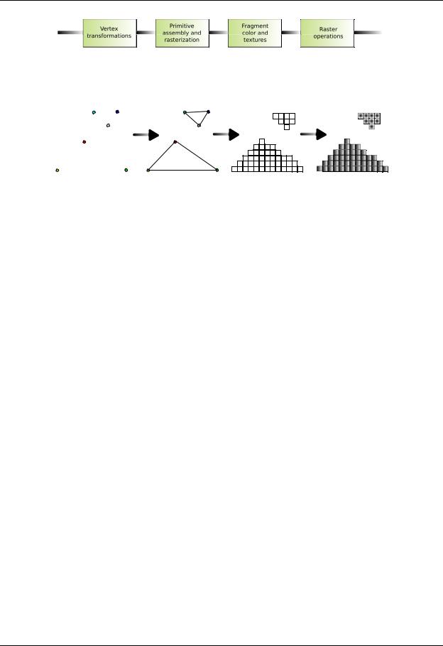
In the graphics pipeline, the graphics application sends a sequence of vertexes, grouped in geometric primitives (polygons, lines and points) that are treated sequentially through the following four di erent stages (see Figure 2.2):

Vertex transformation

Vertex transformation is the first stage of the graphics pipeline. Basically, a series of mathematical operations is performed on each vertex provided by the application (transformation of the position of the vertex into an on-screen position, coordinate generation for the application of textures and color assignation to each vertex,. . . ).

Primitive assembly and Rasterization

The transformed vertices generated from the previous stage are grouped into geometric primitives using the information gathered from the application. As a result, a sequence of triangles, lines or points is obtained. Those points are then passed to a subsequent sub-stage called rasterization. The rasterization is the process by which the set of pixels “covered” by a primitive is determined.

It is important to correctly define the concept of fragment, as it is transformed into a concept of critical importance for general-purpose computations. A pixel location and information regarding its color, specular color and one or more sets of texture coordinates are associated to each fragment.

20

2.1. THE GRAPHICS PIPELINE

Figure 2.3: Detailed graphics pipeline with programmable stages (in red).

In particular, it is possible to view a fragment as a “potential pixel”: if the fragment successfully passes the rest of the pipeline stages, the pixel information will be updated as a result.

Interpolation, Textures and Colors

Once the rasterization stage is complete, and a number of fragments have been extracted from it, each fragment is transformed by interpolation and texture operations (that will result in the most interesting phase for general-purpose computation) and the final color value is determined. In addition to the final coloring of the fragment, this stage is also responsible of discarding a given fragment to prevent its value from being updated in memory; thus, this stage produces either one or zero output fragments for each input fragment.

Last stages

In the final stages of the pipeline, the raster operations process each fragment with a set of tests to evaluate its graphical properties. These tests determine the values that the new pixel will receive from the original fragment. If any of these tests fails, the corresponding pixel is discarded. If all tests succeed, the result of the process is written to memory (usually referred as the framebu er).

2.1.1.Programmable pipeline stages

Until the late 1990s, the way GPUs implemented the logical graphics pipeline consisted on a fixed-function physical pipeline that was configurable, but not fully programmable in any of its parts. The revolution started in 2001 with the introduction of the NVIDIA Geforce 3 series. This was the first graphics processor that provided some level of programmability in the shaders, and thus it o ered the programmer the possibility of personalizing the behavior of some of the stages of the pipeline. NVIDIA Geforce 3 followed the Microsoft DirectX 8 guidelines [19], which required that compliant hardware featured both programmable vertex and pixel processing units.

Nevertheless, the novel generations of GPUs still exhibited separated types of processing units (also called shaders) for the vertex and the pixel processing, with di erent functionality and programming capabilities (see Figure 2.3). In general, the fragment processors were employed for GPGPU programming. First, because they were more versatile than the vertex processors. Second, because the number of fragment processors was usually larger than that of vertex processors.

21