3.4. EXPERIMENTAL RESULTS

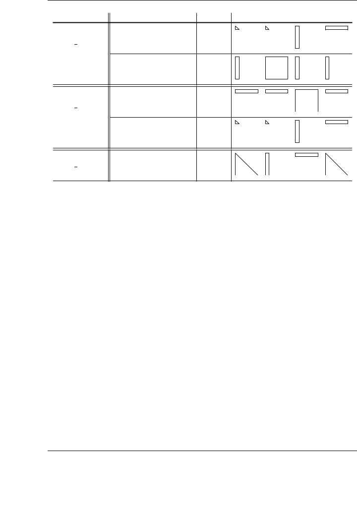
The name of each algorithm describes the shape of the sub-matrices of A and AT that appear as input operands in the operations performed in each iteration of the blocked algorithm. Three di erent algorithmic variants of the SYRK routine are proposed:

Matrix-panel variant (SYRK MP): For each iteration, the computation involves a panel of AT (AT1 ) and a sub-matrix of A, to obtain a panel of columns of C.

Panel-matrix variant (SYRK PM): For each iteration of the panel-matrix variant, a panel of rows of matrix A (A1) is multiplied by a sub-matrix of AT , to obtain a new panel of rows of C.

Panel-panel variant (SYRK PP): In the panel-panel variant a panel of columns of matrix A and a panel of rows of matrix AT are multiplied to update the whole symmetric matrix C at each iteration.

The di erent performances attained by each algorithmic variant of the SYRK routine exposed in Figure 3.11 are dictated by the specific routines invoked in each iteration and, more precisely, by the specific of exploitation of the underlying hardware derived from the di erent shapes of the operands involved. As an example, consider the di erences between the matrix-panel and the panel-matrix variants:

In each iteration of the matrix-panel variant, two invocations to BLAS-3 routines are performed to update the current block of columns of the result matrix C. The first operation, C11 := C11 − A1AT1 , updates the diagonal block C11, and thus is performed by a SYRK routine invocation. The second operation, C21 := C21 − A2AT1 , is cast in terms of GEMM.

For the panel-matrix algorithm, the SYRK invocation is executed on the same block, but the GEMM updates the panel of rows C01.

Although the same routines are invoked in the two variants, the di erence resides in the shapes of the operands of routine GEMM, a critical factor as we have shown. While in the matrix-panel variant a matrix (A2) is multiplied by a panel of columns of matrix AT (AT1 ) to update a panel of columns of matrix C (C21), in the panel-matrix variant, a panel of rows (A1) is multiplied by a matrix (AT0 ) to update a panel of rows of the matrix C (block C10 in the FLAME algorithm). Table 3.5 summarizes the operations and shapes involved in each algorithmic variant of the blocked SYRK implementation.

It is also possible to derive di erent algorithmic variants for the rest of the BLAS-3 routines. Specifically, three di erent variants, analogous to the matrix-panel, panel-matrix and panel-panel variants shown for the GEMM and the SYRK routines, have also been developed for routines SYMM, SYR2K, TRMM, and TRSM; see Figures A.1 to A.4.

3.4.Experimental results

By using the FLAME methodology, an implementation of one case1 for each kernel of the Level- 3 BLAS has been developed and evaluated. The new codes follow a high-level approach, invoking existing NVIDIA CUBLAS routines much in the line of higher-level libraries such as LAPACK. Therefore, no low-level programming is performed to tune the final codes. As an advantage of

1We consider a CASE as a given combination of the available parameters in each BLAS routine.

61

CHAPTER 3. BLAS ON SINGLE-GPU ARCHITECTURES

this approach, the development process to attain high performance codes is made easier, while simultaneously, a full family of algorithms is at the disposal of the developer to choose the optimal one for each specific routine, and each specific case for that routine. The conclusions extracted from the algorithmic perspective (basically optimal algorithmic variants and best block sizes) can be directly applied to lower level codings, such as the native CUDA implementations in which the

62

3.4. EXPERIMENTAL RESULTS

Table 3.5: Operations and shapes of the operands involved in the blocked SYRK algorithmic variants. The partitionings assumed for each variant are those described in Figure 3.11.

NVIDIA CUBLAS routines are based. As an additional advantage, any internal improvement in the performance of the underlying implementation has an immediate impact on the final performance of the developed BLAS routines. Thus, direct performance improvements in the new implementations are expected as future tuned implementations of the GEMM routine are released by NVIDIA or by the scientific community.

The FLAME algorithms derived for each BLAS-3 routine expose two di erent lines of study to be considered to achieve high performance. For example, see the algorithms for the SYRK routine shown in Figure 3.11. First, the block size b must be chosen before the blocked algorithm begins. Second, di erent algorithmic variants must be considered in order to achieve the most suitable ones.

3.4.1.Impact of the block size

In addition to the particular algorithmic variant chosen, the block size is a critical parameter in the final performance of blocked algorithms in general, and particularly important for the blocked variants of the BLAS-3. The influence of the matrix dimensions on the performance the GEMM routine in NVIDIA CUBLAS (see in Figure 3.4) is a clear indicator of its capital importance in the final performance of the new routines. Many internal particularities of the hardware are directly related to this di erences in performance, and they have a visible impact with the modification of the block size (internal memory organization, cache and TLB misses, memory alignment issues, etc.). From the programmer perspective, the ability to easily and mechanically evaluate the e ect of the block size from a high-level point of view implies the possibility of extracting conclusions before the low-level programming e ort begins. The insights extracted for the optimal block size

63

CHAPTER 3. BLAS ON SINGLE-GPU ARCHITECTURES

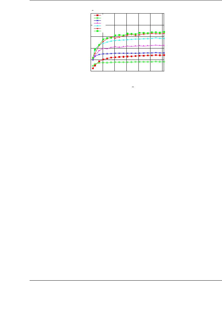
Figure 3.12: Performance of the new, tuned SYRK MP implementation for multiple block sizes.

from this high-level approach are valid and can be applied (if desired) to low-level programming, driving to a faster code optimization.

As an illustrative example, Figure 3.12 shows the di erences in performance for the panelmatrix variant of the SYRK routine using di erent block sizes. There are significant di erences in the performance of the implementation depending on the block size. In general, the GFLOPS rates increase with the size of the block. This improvement is more important when using small blocks and is reduced as the tested block size is close to the optimal one. Figure 3.12 only reports performances for block sizes up to the optimal one; for larger block sizes, the performance rates are usually sustained and the performance does not improve. Observe in the figure the important performance di erence depending on the selected block size. While 80 GFLOPS are attained for a block size b = 32, increasing this value to b = 384 boosts e ciency up to 320 GFLOPS. This speedup (4×), obtained just by varying the block size, gives an idea of the importance of a thorough evaluation of this parameter when operating with blocked algorithms.

A detailed study of the impact of the block size has been carried out for each implementation. The performance results shown for every routine include the performance for the optimal block size from a whole set of block sizes.

3.4.2.Performance results for di erent algorithmic variants

The way in which calculations are organized in a given variant also plays a fundamental role in the final performance of the BLAS implementation. Once again, from the programmer perspective, having a family of algorithmic variants, and systematically evaluating these variants for each specific routine usually guides to a highly tuned implementation. Moreover, this methodology o ers a way to guide the low-level programming e ort to the appropriate parameters by performing a high-level previous evaluation of them.

Note that each implementation of the algorithmic variants for the BLAS routines is based on an initial partitioning and successive repartitioning processes. These partitionings basically translate into movements of pointers in the final codes, so no significant overhead is expected from them. For each iteration, the NVIDIA CUBLAS routines indicated in the FLAME algorithms are invoked, depending on the corresponding routine and algorithmic variants; these routines operate with the sub-blocks of the input and output matrices determined by the former partitioning processes.

64

3.4. EXPERIMENTAL RESULTS

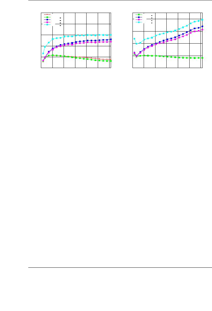
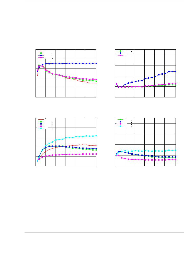
Figure 3.13: Performance (left) and speedup (right) of the three variants for the SYRK implementation.

For each evaluated routine, we compare the corresponding NVIDIA CUBLAS implementation and each new algorithmic variant. The speedup of the new codes is also shown, taking the NVIDIA CUBLAS performance of the routine as the reference for the comparison.

Figures 3.13 to 3.16 report the performance results for the evaluated BLAS routines and cases, and compare the performance of our new implementations with those from NVIDIA CUBLAS. The plots in the left of those figures show raw performances in terms of GFLOPS. The plots in the right illustrate the speedups attained by the new implementation of the routines taking the NVIDIA CUBLAS performance as the base for the calculation. As the block size is a critical factor in this type of blocked algorithms, a full evaluation of the performance of the routines has been carried out. Performance results only illustrate the performance attained with the optimal block size.

The performance behavior of the new implementations for the BLAS SYRK routine shown in Figure 3.13 is representative of the benefits that are expected from the new implementations. The advantages of our new GEMM-based implementations are demonstrated by observing the performances of the matrix-panel and the panel-matrix variants (especially the latter) that delivers a speedup near 2.5× for the largest matrices tested. This speedup is similar for smaller matrices. The performance of the matrix-panel variant is optimal for smaller matrices, but yields poorer performances for the largest matrices tested. This decreasing performance agrees with the behavior of the matrix-matrix multiplication shown in the GEMM evaluation (see Figure 3.3 for the case C := C + ABT , in which this variant of the SYRK operation is based). Similar conclusions and performance results for the SYR2K and the TRMM routines are shown in Figure 3.15. The cases analyzed for each routine are the same as those used for the evaluation of NVIDIA CUBLAS in Section 3.2.1.

In general, for each new implementation there is at least one algorithmic variant that improves significantly the performance of the original NVIDIA CUBLAS implementations. The systematic evaluation of several algorithmic variants, and a detailed study of other critical parameters, such as block sizes, o er a set of conclusions related to the optimal algorithm and parameters for each specific routine, and drive to remarkable speedups for all BLAS routines compared with NVIDIA CUBLAS. As an example, the maximum speedup is 4× for SYMM, and the performance of the new implementations is higher than 300 GFLOPS for all implemented routines.

Further optimizations are possible from the basic algorithmic variants. For example, the performance of the SYMM implementations su ers from the poor performance of the NVIDIA CUBLAS

65

CHAPTER 3. BLAS ON SINGLE-GPU ARCHITECTURES

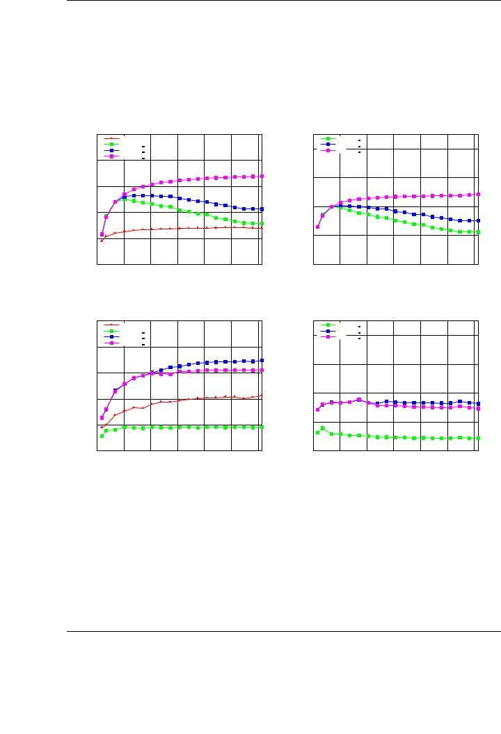
Figure 3.14: Performance (left) and speedup (right) of the three variants for the SYMM implementation.

SYMM implementation in all its algorithmic variants (see the performances of the basic algorithmic variants in Figure 3.14). Our basic SYMM implementation attains near 250 GFLOPS for the best variant, while the speed of the rest of our tuned implementations varies between 300 and 350 GFLOPS. Taking as reference the panel-matrix variant shown in Figure A.1, it is possible to observe that the operation involving a diagonal block of the input matrix A (block A11 in the algorithm) is the only one cast in terms of NVIDIA CUBLAS SYMM, which becomes the key bottleneck for the performance of the implementation.

A possible approach to this problem is to use an additional workspace to store the diagonal block of A in its full form, instead of storing only the lower triangular part. To do so, the algorithm has to explicitly copy the contents from the lower triangular part of the block into the upper triangular part, creating a symmetric matrix. Proceeding in this way, the operation C1 := C1 + A11B1, with A11 a block considered symmetric and stored in compact scheme, is symmetrized into the operation

in GPU memory. Thus, this operation can be cast exclusively in terms of a GEMM instead of using SYMM to perform it, potentially boosting the performance. The performance attained by this optimization based con the panel-matrix variant is also shown in Figure 3.14; in essence, proceeding this way a blocked general matrix-matrix multiplication is finally performed, introducing a small penalty related to the allocation of the workspace and the transformation of the compact symmetric matrix into canonical storage. This explains the di erence in performance of this implementation compared with the performance of the NVIDIA CUBLAS GEMM implementation shown in Figure 3.3. Similar techniques can be applied to the rest of the routines involving symmetric matrices (SYRK and SYR2K).

One of the benefits of the GEMM-based approach is the direct impact of the inner-kernel (in this case, the GEMM routine) in the final performance of the rest of the BLAS implementations. For example, consider the performance of the NVIDIA CUBLAS implementation for the GEMM operation when matrix B is transposed; see Figure 3.16. As can be observed, the NVIDIA CUBLAS implementation performs particularly poor for large matrix sizes. We have developed blocked algorithms for this operation following the algorithms outlined in Figure 3.8, identifying a variant (the panel-matrix one) that performs particularly well, attaining a speedup 2.5× compared to the basic NVIDIA CUBLAS implementation for matrices of large dimension.

66

3.4. EXPERIMENTAL RESULTS

Figure 3.15: Top: performance (left) and speedup (right) of the three variants for the SYR2K implementation. Bottom: performance (left) and speedup (right) of the three variants for the TRMM implementation.

67

CHAPTER 3. BLAS ON SINGLE-GPU ARCHITECTURES

Figure 3.16: Top: Performance (left) and speedup (right) of the three variants for the GEMM implementation. Bottom: Performance (left) and speedup (right) of the three variants for the TRSM implementation.

68