5.4. EXPERIMENTAL RESULTS

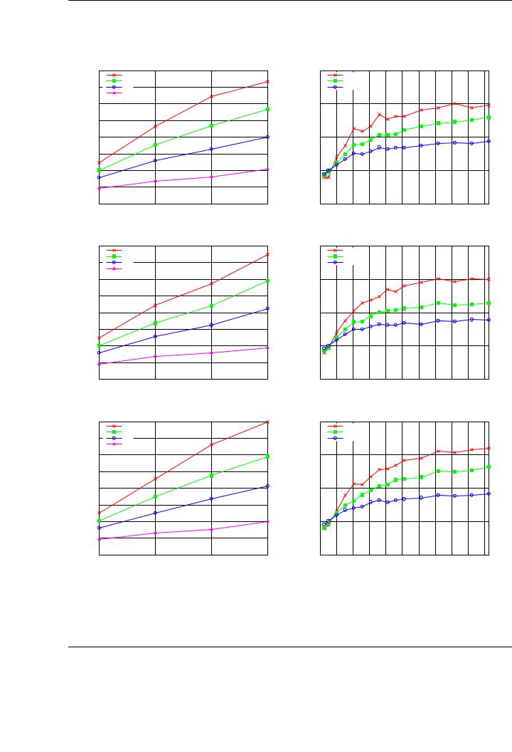
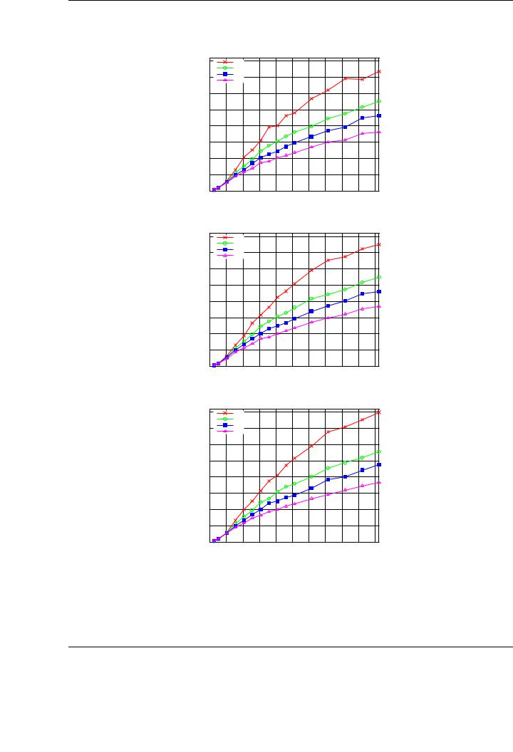
Figure 5.9 shows the performance attained for the Cholesky factorization of a matrix of increasing size on the four versions of the runtime, with 2-D data distribution for versions 2-4. The plots show the performance of the algorithmic variants (Variant 1 in the top plot, Variant 2 in the middle plot and Variant 3 in the bottom plot).

A careful observation of the performance results o ers an idea of the impact of the reduction of data transfers while improving data transfer management. As an starting point, consider in the following discussion the results attained for Variant 1 of the algorithm. Peak performance for the basic implementation (Version 1 of the runtime), in which data is transferred to GPU memory prior to the execution of the task and retrieved back after its conclusion, is 357 GFLOPS. The usage of data a nity and the storage of own blocks in the corresponding GPU (Version 2 of the runtime) boosts this performance up to 467 GFLOPS. With the introduction of the software cache mechanism with a write-through coherence policy between main memory an GPU memory (Version 3 of the runtime) performance is increased to 544 GFLOPS. Finally, the use of a combination of software cache and a write-back policy is translated into the best raw performance, attaining a peak of 705 GFLOPS. Note that this performance is not still fully stabilized, and could be further increased for larger matrices, provided there was enough memory space in the aggregated GPU memory space.

Similar qualitative results and improvements are shown for algorithmic variants 2 and 3 (middle and bottom plots, respectively). The speedup ratios are similar to those achieved for the first variant using di erent runtime versions. Considering raw performance, variant 3 attains a peak performance of 798 GFLOPS, whereas variants 1 and 2 achieve 735 GFLOPS and 751 GFLOPS, respectively. As was the case in the evaluation of single-GPU implementations, these results demonstrate the benefits of providing a whole family of algorithmic variants for multi-GPU systems in order to find the optimal one for a given operation.

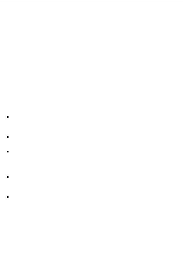
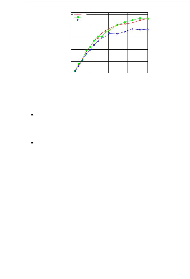
To analyze the scalability of the proposed software solution, in Figure 5.10 we evaluate the scalability (left-hand side plots) and reports the speed-up (right-hand side plots) of the di erent algorithmic variants of the algorithm-by-blocks.

As an illustrative example, consider the top plot, which corresponds to the algorithmic variant 1. No bottlenecks are revealed in the scalability of this variant: the performance of the system steadily improves as the number of GPUs is increased, and larger problem sizes report higher execution rates. The speed-ups are calculated comparing the performance attained by the algorithms-by-blocks using 2–4 GPUs with that of executing same algorithm on a single graphics processor. For the largest problem dimension, the results show speed-ups of 1.9×, 2.5×, and 2.9× using respectively 2, 3, and 4 GPUs for variant 1; 1.7×, 2.2×, and 3× for variant 2; and 1.8×, 2.6×, and 3.2× for variant 3. Note that the PCI-Express bus becomes a bottleneck as the number of GPUs increases. This justifies the necessity of a proper data transfer policy as those implemented in our runtime.

5.4.4.Impact of data distribution

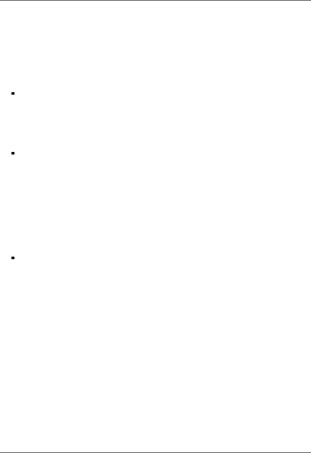
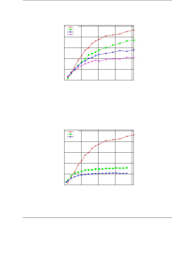
Data layout is an additional factor that can a ect the performance attained for a given operation using any of the tuned variants of the developed runtime. The performance di erences are mostly explained by a higher data locality when using runtime versions that make use of software caches.

Figure 5.11 shows the performance of the proposed algorithmic variants for the Cholesky factorization using the four GPUs of TESLA2, and version 4 of the runtime. The experimental conditions are the same as those set in previous experiments. In this experiment, we report the performance results attained for three di erent data distributions: cyclic 2-dimensional (top plot), column-wise distribution (middle plot) and row-wise distribution (bottom plot).

151

CHAPTER 5. MATRIX COMPUTATIONS ON MULTI-GPU SYSTEMS

Cholesky factorization on TESLA2. 2-D distribution. Variant 1

Matrix size

Cholesky factorization on TESLA2. 2-D distribution. Variant 2

Matrix size

Cholesky factorization on TESLA2. 2-D distribution. Variant 3

Matrix size

Figure 5.9: Performance comparison of di erent algorithmic variants of the Cholesky factorization using 4 GPUs on TESLA2, using a 2-D distribution. Top: algorithmic variant 1. Middle: algorithmic variant 2. Bottom: algorithmic variant 3.

152

5.4. EXPERIMENTAL RESULTS

Figure 5.10: Scalability (left) and speedup (right) of the Cholesky factorization on TESLA2.

153

CHAPTER 5. MATRIX COMPUTATIONS ON MULTI-GPU SYSTEMS

For the specific algorithmic variant implemented, the data distribution policy can play an important role on the final performance of the parallel implementations, especially for large matrices.

Variant 3 is the most e cient algorithmic variant independently from the selected data distribution, with negligible performance di erences among them. On the other hand, consider the performance of Variant 3 for di erent data distributions and a large matrix dimension (n = 20,480). In this case, the performance attained by the runtime-based implementation varies from 741 GFLOPS for the 2-D cyclic distribution, to 753 GFLOPS for the column-wise layout and down to 625 GFLOPS for the row-wise distribution. Although smaller, there are also subtle di erences in the performance of Variant 1 depending on the chosen data distribution.

The conclusion of this experiments is that spatial assignment of data (and therefore, tasks) to GPUs is also an important factor with relevant impact on the final performance, much like algorithmic variant, block size and data transfer policy were revealed in previous experiments. A careful study of this parameter becomes critical to achieve optimal results for every operation.

5.4.5.Performance comparison with other high-performance implementations

In order to gain a better understanding of previous results for the multi-GPU setup, Figure 5.12 compares the performances of the algorithm-by-blocks for the Cholesky factorization with those of optimized implementations of these operations on current high-performance platforms:

Algorithm-by-blocks on four GPUs: Our algorithm-by-blocks for the Cholesky factorization, using the version 4 of the runtime system, and executed on TESLA2 using the four available GPUs.

Algorithm-by-blocks on one GPU: Our algorithm-by-blocks for the Cholesky factorization, using the version 4 of the runtime system, and executed on TESLA2 using only one GPU.

Blocked-algorithm on one GPU: Implementation of the hybrid Cholesky algorithm as presented at Chapter 4 on a single GPU of TESLA2. To be consistent with previous results, the time to transfer the data from main memory to GPU memory and retrieve the results is included.

Algorithm-by-blocks on the multi-core processors of TESLA2: Our algorithms-by-blocks for the Cholesky factorization, using the SuperMatrix runtime system [45], and executed on TESLA2 using the its eight cores.

MKL spotrf on the multi-core processors of TESLA2: A multi-threaded implementation of the corresponding LAPACK routine executed using the eight cores of TESLA2.

The benefits of using the runtime-based approach can be derived by comparing the performance results on 4 GPUs with those obtained for one GPU using the blocked algorithm. More precisely, the performance is increased from 267 GFLOPS for the mono-GPU blocked implementation to roughly 800 GFLOPS for the multi-GPU implementation.

In addition, the overhead introduced by the runtime is not important, as can be realized by comparing the results for the mono-GPU implementations using the blocked algorithm and the algorithm-by-blocks combined with the runtime (267 GFLOPS for the first implementation and 249 GFLOPS for the runtime-based implementation, for the largest tested matrices). The lack of code modifications to deal with multi-GPU systems further justifies the usage of the runtime-based approach and validates the solution also for mono-GPU architectures.

154

5.4. EXPERIMENTAL RESULTS

Cholesky factorization on TESLA2. 2-D distribution

Matrix size

Cholesky factorization on TESLA2. Column-wise distribution

Matrix size

Cholesky factorization on TESLA2. Row-wise distribution

Matrix size

Figure 5.11: Performance comparison of di erent algorithmic variants of the Cholesky factorization using 4 GPUs on TESLA2. Top: 2-D distribution. Middle: column-wise distribution. Bottom: row-wise distribution.

155

CHAPTER 5. MATRIX COMPUTATIONS ON MULTI-GPU SYSTEMS

Cholesky factorization on GPUs and multi-core on TESLA2

Matrix size

Figure 5.12: Performance of the Cholesky factorization using GPUs and multi-core on TESLA2.

The algorithm-by-blocks using the SuperMatrix runtime roughly attains 150 GFLOPS using the 8 cores in TESLA2. This figure shows how, with minor modifications in the FLAME codes, performance can be boosted from 150 GFLOPS to 800 GFLOPS by using the GPUs as the underlying architecture, implementing the same algorithm-by-blocks. Comparing the implementation of the algorithm-by-blocks with the optimized implementation in MKL gives an idea of the benefits of this type of algorithms, as the optimized library only attains 70 GFLOPS for the Cholesky factorization using the same experimental setup.

5.5.Multi-GPU implementations for the BLAS

The Cholesky factorization is an appropriate example to illustrate the possibilities of a runtime system like that developed for multi-GPU systems. The algorithm-by-blocks exhibits a number of characteristics that are appealing to exploit the benefits of the improvements introduced in the runtime (heterogeneity in the type of tasks, multiple data dependencies, use of the CPU or the GPU depending on the specific task type,. . . ).

In this section, we report and analyze the performance results for three common BLAS routines, implemented using algorithms-by-blocks and on a multi-GPU system. These results illustrate how a common run-time system can be used as the base for several implementations, o ering appealing performance results without a ecting the programmability of the solution. In fact, the developed system can be applied to obtain a full BLAS implementation for multi-GPU systems, without any modification on existing algorithms-by-blocks for the routines.

Although minor new insights can be extracted from a deep analysis of the performance results for BLAS routines, the major part of the observations were already gained from the experimentation with the Cholesky factorization. Thus, we focus on reporting experimental results, comparing them with other high-performance implementations on systems with one GPU and/or multi-core architectures when possible. The main goal is to illustrate how the approach based on a runtime and minor modifications to the original FLAME code can be applied to a wide variety of linear algebra routines with appealing performance results.

156

5.5. MULTI-GPU IMPLEMENTATIONS FOR THE BLAS

5.5.1.Triangular system solve (TRSM)

The TRSM routine is a challenging implementation on multi-GPU platforms, since it presents a rich variety of data dependencies. In this case, we evaluate a particular case of the TRSM routine, even though similar results are expected for other cases.

In this case, the evaluation focuses on XAT = B, where A is lower triangular and B is overwritten with the solution X. We show performance results obtained by performing three di erent experiments:

Evaluation of the performance of the runtime versions: Figure 5.13 shows the performance of the TRSM implementation executed on 4 GPUs of TESLA2. The figure shows results for the four versions of the developed runtime. Like was the case for the Cholesky factorization, the reduction in the number of data transfers plays a significant role in the final performance of the parallel implementation. Performance results vary from 416 GFLOPS using Version 1 of the runtime up to 926 GFLOPS for version 4.

Comparison to single-GPU implementations: Figure 5.14 shows a comparison of the performance of the multi-GPU implementation using the run-time system with two di erent monoGPU implementations. The first one is the implementation o ered by NVIDIA CUBLAS. The second one is the best implementation described in Chapter 3. For the largest matrices that a single GPU can hold, 206 GFLOPS are attained using NVIDIA CUBLAS on one GPU, 320 GFLOPS using our own implementation of the routine on one GPU, and 900 GFLOPS using the most tuned version of the runtime and four GPUs. Note that, for small matrices (up to n = 3,072 in the example), the single-GPU implementations are more e cient than the multi-GPU implementations, mainly due to the small amount of parallelism that can be extracted if a block size which is relatively large is chosen to attain high performance in the inner kernels.

Impact of the layout on the performance: Unlike the conclusions extracted for the Cholesky factorization (see Figure 5.11), data distribution plays a fundamental role in the TRSM implementation on multi-GPU architectures. Figure 5.15 shows the performance of version 4 of the runtime using the 4 GPUs of TESLA2, for three di erent data distributions: 2-D cyclic, row-wise and column-wise. As reported in the plot, there are minor performance di erences between the 2-D cyclic distribution and the row-wise distribution. However, the di erence in performance between those two and the column-wise distribution is remarkable: 926 GFLOPS are attained for the 2-D cyclic distribution, but this rate is reduced to 731 GFLOPS for the column-wise distribution.

Multi-GPU implementations often deliver high gains for problems of large dimension. For instance, consider the TRSM performance in Figure 5.14. For a moderate matrix dimension (n = 5,120), single-GPU implementations achieve a performance rate that is close to the peak achieved for the largest tested matrix. However, the performance rate attained on 4 GPUs is still half of that attained for the largest matrix tested (425 GFLOPS vs. 926 GFLOPS). This is a frequent behavior of multi-GPU implementations and finally determines whether this type of architectures is appropriate to tackle a given problem depending on its size.

5.5.2.Symmetric rank-K update (SYRK)

The next study is focused on a representative case of this operation, C := C − AAT , where C is symmetric and only the lower triangular part of this matrix is stored and computed. We carry

157

CHAPTER 5. MATRIX COMPUTATIONS ON MULTI-GPU SYSTEMS

TRSM on 4 GPUs on TESLA2

Matrix size

Figure 5.13: Performance of the TRSM implementation using 4 GPUs on TESLA2.

TRSM implementations on TESLA2

Matrix size

Figure 5.14: Performance of several TRSM implementations on TESLA2.

158

5.5. MULTI-GPU IMPLEMENTATIONS FOR THE BLAS

Data distribution pattern for the TRSM implementation on TESLA2

Matrix size

Figure 5.15: Impact of the data distribution pattern on the TRSM implementation on TESLA2.

out the analysis for operations with square matrices, although similar results are expected for other experimental configurations.

Evaluation of the performance of the runtime versions: Figure 5.16 (left) reports the performance of the developed versions of the runtime for the SYRK routine on four GPUs of TESLA2. The performance results validate the successive refinements introduced in the runtime to reduce data transfers. Performance is increased from 402 GFLOPS in the basic version of the runtime to almost 1 TFLOP using the most sophisticated version.

Comparison to mono-GPU implementations: Figure 5.16 (right) compares the best result attained using the run-time system on the multi-GPU setup (with four GPUs) with two di erent implementations of mono-GPU codes: the NVIDIA CUBLAS implementation and our own tuned implementation using blocked algorithms. The benefits of the run-time system are clear: for the largest tested matrices, performance is increased from 161 GFLOPS o ered by NVIDIA CUBLAS and 321 GFLOPS of our tuned implementation to 965 GFLOPS of the multi-GPU configuration using the runtime on the four GPUs of TESLA2. Once more, the multi-GPU setup shows its potential for relatively large matrices, where distributing the computation among several GPUs is more appropriate.

5.5.3.Matrix-matrix multiplication (GEMM)

The matrix-matrix multiplication is usually evaluated on novel systems and its performance shown as illustrative of the performance that can be attained by the architecture. Following this trend, we report performance results for a specific case of matrix-matrix multiplication using our run-time system on TESLA2.

The study considers the particular case C := C − ABT , where A, B, and C are square matrices. Similar results are expected for other experimental configurations. For this evaluation, we skip the detailed report of the performance o ered by the di erent versions of the runtime, as the insights

159