CHAPTER 4. LAPACK-LEVEL ROUTINES ON SINGLE-GPU ARCHITECTURES

Table 4.1: Time breakdown for the factorization of one diagonal block for di erent block sizes on the CPU and on the GPU. Time in ms.

Whether this technique yields a performance gain depends on the overhead due to the data transfer between GPU and main memories as well as the performance of the Cholesky factorization of small matrices on the multi-core CPU.

To evaluate the impact of the intermediate data transfers, Table 4.1 analyzes the time devoted to intermediate data transfers to and from GPU memory necessary for the factorization of the diagonal block on the CPU. As shown, there is a major improvement in the factorization time for the tested block sizes on the CPU, even taking into account the necessary transfer times between memories (compare the columns “Total CPU”, that includes data transfer times, with the column “Fact. on GPU”).

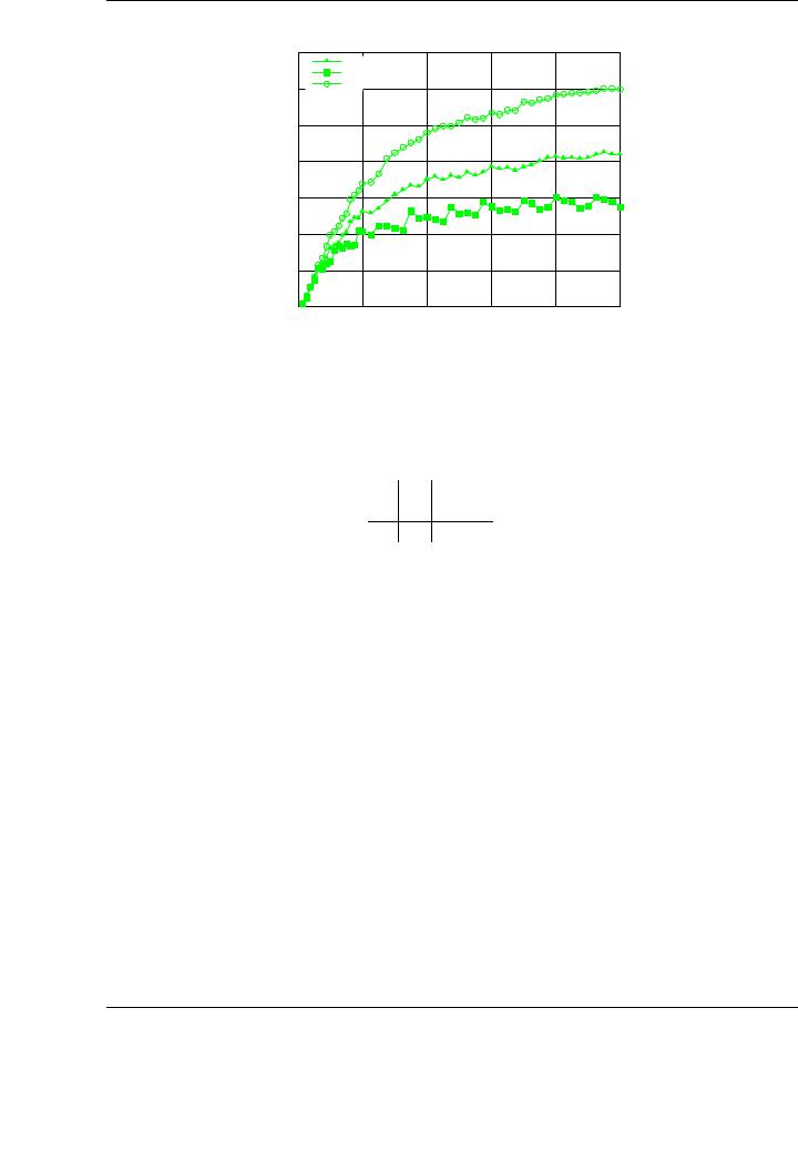
Figure 4.8 reports the performance of the hybrid version of the blocked Cholesky algorithmic variants. Diagonal blocks are factorized using the multi-threaded MKL implementation, using the 8 cores of the architecture. The rest of the experimental setup is identical to that used in previous experiments.

The benefits of the hybrid approach are clear from the observation of the figure. With independence of the chosen variant, performance is improved compared with the rates attained for the padded variants (compare Figures 4.7 and 4.8). For example, Variant 3 of the blocked Cholesky factorization attains 241 GFLOPS in the version executed exclusively on the GPU and 301 GFLOPS in the hybrid version.

4.4.LU factorization

The LU factorization, combined with a pivoting strategy (usually partial row pivoting) is the most common method to solve linear systems when the coe cient matrix A does not present any particular structure. As for the Cholesky factorization, a necessary property of the coe cient matrix A is to be invertible.

The LU factorization of a matrix A Rn×n involves the application of a sequence of (n − 1) Gauss transformations [144], that ultimately decompose the matrix into a product A = LU, where L Rn×n is unit lower triangular and U Rn×n is upper triangular.

90

4.4. LU FACTORIZATION

Figure 4.8: Performance of the single-precision blocked algorithmic variants of the Cholesky factorization on the graphics processor using padding and a hybrid execution approach

on PECO.

Definition A Gauss transformation is a matrix of the form

0l21 In−i−1

An interesting property of the Gauss transformations is how they can be easily inverted and applied. The inverse of the Gauss transformation in (4.1) is given by

while, for example, applying the inverse of L0 to a matrix A boils down to

The main property of the Gauss transformations is the ability to annihilate the sub-diagonal elements of a matrix column. For example, taking l21 := a21/α11 in (4.3), we have a21 − α11l21 = 0, and zeros are introduced in the sub-diagonal elements of the first column of A.

Another interesting property of the Gauss transformations is that they can be easily accumulated, as follows:

where L00 Rk×k.

91

CHAPTER 4. LAPACK-LEVEL ROUTINES ON SINGLE-GPU ARCHITECTURES

Considering these properties, it is easy to demonstrate that the successive application of Gauss transformations corresponds in fact to an algorithm that computes the LU factorization of a matrix. Assume that after k steps of the algorithm, the initial matrix A has been overwritten with

. . . L−1 1L−0 1A, where the Gauss transformations Lj, 0 ≤ j < k ensure that the sub-diagonal

Proceeding in this way, it is possible to reduce a matrix to an upper triangular form by successively applying Gauss transformations that annihilate the sub-diagonal entries, which e ectively computes an LU factorization. Note that if L−n−1 1 . . . L−1 1L−0 1A = U, then A = LU, where L = L0L1 . . . Ln−1 is built from the columns of the corresponding Gauss transformations.

Once the coe cient matrix is decomposed into the corresponding triangular factors, it is possible to obtain the solution of the linear system Ax = b by solving two triangular systems: first, the solution of the system Ly = b is obtained using progressive elimination; and then the system Ux = y is solved by regressive substitution. As for the Cholesky factorization, these two stages involve lower computational cost, and thus the optimization e ort is usually focused on the factorization stage.

To summarize, the LU factorization decomposes a matrix A into a unit lower triangular matrix L and an upper triangular matrix U such that A = LU. The following theorem dictates the conditions for the existence of the LU factorization.

matrices AT L, 1 ≤ k ≤ n, are called the leading principle sub-matrices of A.

The proof for this theorem can be found in the literature; see [70].

92

4.4. LU FACTORIZATION

4.4.1.Scalar algorithm for the LU factorization

This section describes, using a formal derivation process, a scalar algorithm to obtain the LU factorization of a matrix A Rn×n. During this process, the elements below the diagonal of L overwrite the strictly lower triangular part of A, while the elements of U overwrite its upper triangular part. The diagonal of L is not explicitly stored as its elements are all 1.

Consider the following partitionings for the coe cient matrix A and its factors L and U:

where α11 and µ11 are scalars, a21, l21, and u12 vectors of n − 1 elements, and A22, L22 and U22 matrices of size (n − 1) × (n − 1). From A = LU,

and the following expressions are derived:

Proceeding in this manner, a recursive formulation of a scalar algorithm for the LU factorization is obtained; in this formulation, the elements of A are overwritten with those from the factors L and U as follows:

2.α11 := µ11 = α11.

3.aT12 := uT12 = aT12.

4.a21 := l21 = a21/µ21.

5.A22 := A22 − l21uT12.

6.Continue recursively with A = A22 in step 1.

The scalar algorithm to calculate the LU factorization presents a computational cost of 2n3/3 flops. As in the Cholesky factorization, the major part of the calculation is due to the rank-1 update, that involves O(n2) arithmetic operations on O(n2) data. As usual, it is convinient to reformulate the algorithm in terms of operations with matrices (or rank-k updates), to improve the ratio between arithmetic operations and memory accesses, allowing a proper data reutilization that exploits the sophisticated memory hierarchy of modern processors. The blocked algorithm presented next pursues this goal.

93