6.3. DENSE LINEAR ALGEBRA LIBRARIES FOR MESSAGE-PASSING PROGRAMMING

Blocks owned by processor (0, 0)

Figure 6.4: Block-cyclic data distribution of a matrix on a 2 × 3 grid of processes

Programmability

This is one of the weakest points of ScaLAPACK. To illustrate a practical example of the usage of ScaLAPACK and establish a base for a comparison with PLAPACK, we show the prototype of the P GEMM function. P GEMM is the PBLAS routine in charge of performing a distributed matrix-matrix multiplication. The interface of this routine is specified as:

The nomenclature and options of the invocations are directly inherited from BLAS and LAPACK. Besides the intricate indexing and dimension handling, parameters DESCx, with x being A, B, or C describe the two-dimensional block-cycling mapping of the corresponding matrix. This array descriptor is an integer array with 9 elements.

The first two entries of DESCx are the descriptor type and the BLACS context. The third and fourth ones denote the dimensions of the matrix (number of rows and columns, respectively). The fifth and sixth entries specify the row and column block sizes used to distribute the matrix. The seventh and eighth entries identify the coordinates of the process containing the first entry of the matrix. The last one is the leading dimension of the local array containing the matrix elements.

This syntax gives an idea of the complex usage of ScaLAPACK as a library. The programmer is not abstracted from data distributions. Many of the parameters managed internally by ScaLAPACK have to be explicitly handled by the programmer.

The usage of ScaLAPACK as an infrastructure to build new routines is also possible. In that case, complexity appears in the usage of BLACS and PBLAS as the underlying libraries to support communication and parallel execution. The description of those software elements is out of the scope of this dissertation. Further information can be found in the ScaLAPACK documentation.

6.3.2.PLAPACK

PLAPACK [137, 18, 7] is a library and an infrastructure for the development of dense and banded linear algebra codes. As a library, it provides the whole functionality of the three BLAS

173

CHAPTER 6. MATRIX COMPUTATIONS ON CLUSTERS OF GPUS

levels, plus some of the functionality at the LAPACK level. As an infrastructure, it provides the necessary tools to allow the library developer to easily implement new distributed-memory routines with relatively small e ort and high reliability. It has been widely used [150, 17, 146, 151] through the years, mainly due to its reliability and ease of programming.

Natural algorithmic description

PLAPACK introduced a methodology for algorithm description, development and coding that was the kernel of the FLAME methodology. Thus, programmability and natural port of algorithm descriptions directly to code lie the foundations of the infrastructure.

The main advantages of the methodology underlying PLAPACK can be easily illustrated by reviewing its implementation of the Cholesky factorization, an operation already introduced in previous chapters (a more detailed PLAPACK implementation of the Cholesky factorization will be given in Section 6.4.2). As in previous chapters, the goal is to illustrate how the algorithmic description of the operation can be translated directly into a code ready to execute on distributedmemory architectures.

The mathematical formulation of the Cholesky factorization of a, in this case, symmetric positive

definite matrix A, given by

A = LLT ,

yields the following steps to obtain the Cholesky factorization, as detailed in previous chapters (assuming that the lower triangular part of A is overwritten by its Cholesky factor L):

1.α11 := λ11 = √α11.

2.a21 := l21 = a21/λ11.

3.A22 := A22 − l21l21T .

4.Compute the Cholesky factor of A22 recursively, to obtain L22.

Three main observations naturally link to the programming style proposed by PLAPACK:

1.The blocks in the algorithms are just references to parts of the original matrices.

2.There is not an explicit indexing of the elements in the original matrix. Instead there is an indexing of parts of the current matrix, not the original one.

3.Recursion is inherently used in the algorithm.

Consider the following fragment of PLAPACK code which can be viewed as a direct translation of the algorithm for the Cholesky factorization:

7Take_sqrt ( a11 );

174

6.3. DENSE LINEAR ALGEBRA LIBRARIES FOR MESSAGE-PASSING PROGRAMMING

First, all the information that describes a distributed matrix (in this case, matrix A), including the information about the layout of its elements among processes is encapsulated in a data structure (or object) referenced in the code by a. From this data structure, multiple references, or views to the whole object (or parts of it) can be created. For example, function PLA Obj view all creates a reference acur to the same data as a. Object properties are extracted to guide the execution of the algorithm. In the example, routine PLA Obj global length extracts the current size of the matrix referenced by acur. In this case, when this value is zero, the recursion ends.

Matrix partitioning is performed in the code with the routine PLA Obj split 4, creating references to each one of the new four quadrants of the original matrix. From these sub-matrices, each one of the operations needed by the algorithm are performed on the corresponding data: Take sqrt obtains the square root of α11, a21 is scaled by 1/α11 by invoking the routine PLA Inv scal and the symmetric rank-1 update of A22 is computed in PLA Syr.

How parallelism is extracted from these operations will be illustrated by means of particular examples in the next sections. Both the internals of those operations and the higher-level implementation shown for the Cholesky factorization deliver a natural transition between the algorithmic essence of the operation and its implementation on distributed-memory architectures.

Data distribution in PLAPACK

PLAPACK was a revolution not only because of the novel programming paradigm that it introduced (that was, in fact, the kernel of the FLAME project), but also because of the approach taken to distribute data among processes. Typically, message-passing libraries devoted to matrix computations distribute data to be processed by initially decomposing the matrix. PLAPACK advocates for a di erent approach. Instead of that, PLAPACK considers how to decompose the physical problem to be solved.

In this sense, the key observation in PLAPACK is how the elements of the vectors involved in the computation are usually related with the significant data from the physical point of view. Thus, distribution of vectors instead of matrices naturally determines the layout of the problem among the processes. For example, consider the linear transform:

y = Ax

Here, matrix A is merely a relation between two vectors. Data in the matrix do not have a relevant significance themselves. The nature of specified by the vector contents.

This insight drives to the data distribution strategy followed by PLAPACK, usually referred to as PMBD or Physically Based Matrix Distribution. The aim is to distribute the problem among the processes, and thus, in the former expression, one starts by partitioning x and y and assigning these partitions to di erent processes. The matrix A can be then distributed consistently with the distribution chosen for the vectors.

We show here the process to distribute vectors and, therefore, derive matrix distributions alike PLAPACK. We start by defining the partitioning of vectors x and y:

175

CHAPTER 6. MATRIX COMPUTATIONS ON CLUSTERS OF GPUS

and

where Px and Py are permutations that order the elements of vectors x and y, respectively, in some given order. In this case, if processes are labeled as P0, . . . , Pp−1, then sub-vectors xi and yi are assigned to process Pi.

Then, it is possible to conformally partition matrix A:

From there, we have that:

Note how this expression shows the natural association between the sub-vectors of Pxx and the corresponding blocks of columns of PyAPxT .

Analogously,

p−1

X

yi = Ai,jxj

j=0

means that there is also a natural association between sub-vectors of Pyy and corresponding blocks of rows of PyAPxT .

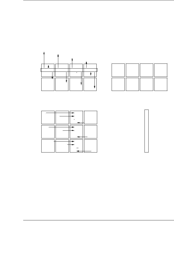
Previous studies [54, 78] concluded that scalability of the solutions is improved if matrices are assigned to processes following a two-dimensional matrix distribution. In this case, the p nodes are logically viewed as a r×c = p mesh. This forces a distribution of sub-vectors to the two-dimensional mesh. PLAPACK uses a column-major order for this distribution. Now, the distribution of matrix A requires that blocks of columns Ai, are assigned to the same column of nodes as sub-vector xj , and blocks of rows Ai, to the same rows of nodes as sub-vector yi, as seen in Figure 6.5.

The figure shows the mechanism used by PLAPACK to induce a matrix distribution from vector distributions. Consider a 3 × 4 mesh of processes, each one represented by a box in the diagram in the top of the figure. Each sub-vector of x and y is assigned to the corresponding node following a column-major ordering. Projecting the indices of y to the left, the distribution of the matrix rowblocks of A is determined. Projecting the indices of x to the top, the distribution of column-blocks

176

6.3. DENSE LINEAR ALGEBRA LIBRARIES FOR MESSAGE-PASSING PROGRAMMING

of A is determined. The diagrams in the bottom show the same information from di erent points of view. In the left-hand side, the resulting distribution of the sub-blocks of A is shown. In the right-hand diagram, the matrix is partitioned into sub-blocks, with the indices in the sub-blocks indicating the node to which the sub-block is mapped.

Data redistribution, duplication and reduction in PLAPACK

Besides computation and data distribution, communication is the third main building block in PLAPACK. The fundamentals of data communication in PLAPACK are based on the mechanisms used to redistribute, duplicate and reduce data. These are the basic operations required to support the complete functionality of the PLAPACK infrastructure.

We illustrate here one example of redistribution, duplication and reduction. Further information and examples can be found in the literature.

Redistribution of a vector to a matrix row. Consider a vector x distributed to the mesh of processes according to the inducing vector for a given matrix A; see Figure 6.6. Observe how blocks of columns of A are assigned to nodes by projecting the indices of the corresponding sub-vectors of the inducing vector distribution.

The transformation of x into a row of matrix A requires a projection onto that matrix row. The associated communication pattern is a gather of the sub-vectors of x within columns of nodes to the row that holds the desired row of A.

The inverse process requires a scatter within columns of A, as shown in Figure 6.6.

For the necessary communication patterns for the redistribution of a vector to a matrix column (and inverse) or a matrix row to a matrix column (and inverse), see [137].

Spread (duplicate) of a vector within rows (or columns) of nodes. Duplication (spread) of vectors, matrix rows or matrix columns within rows or columns of nodes is also a basic communication scheme used in PLAPACK. Upon completion, all rows of nodes or columns of nodes own a copy of the distributed row or column vector.

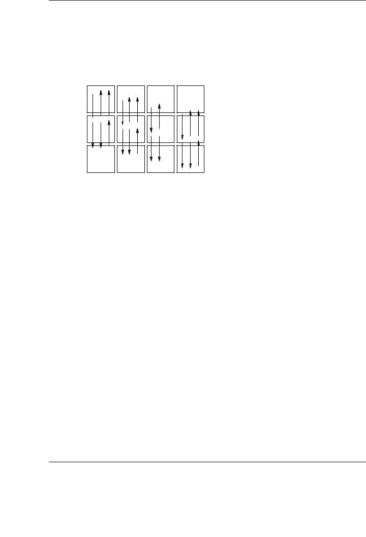
Consider the result of gathering a vector as illustrated in Figure 6.7. If the goal is to have a copy of this column (row) vector within each column (row) of nodes, it is necessary to collect the vector within rows (columns) of nodes, as shown in Figure 6.7.

For the necessary communication patterns for the duplication of a matrix row (or column) within rows (or columns) of nodes, see [137].

Reduction of a spread vector. Given a previously spread vector, matrix row or matrix column, multiple copies of the data coexist in di erent processors. Usually, as part of a distributed operation, multiple instances exist, each one holding a partial contribution to the global result. In that situation, local contributions must be reduced into the global result.

Often, the reduction is performed within one or all rows or columns of the process mesh. Figure 6.8 shows this situation. Consider that each column of processes holds a column vector that has to be summed element-wise into a single vector. In this situation, a distributed reduction of data that leaves a sub-vector of the result on each node has to be performed.

Note how the observations for data consolidation, duplication and reduction yield a systematic approach to all possible data movement situations in PLAPACK.

177

CHAPTER 6. MATRIX COMPUTATIONS ON CLUSTERS OF GPUS

Figure 6.5: Induction of a matrix distribution from vector distributions. (a) Sub-vectors of x and y distributed to a 3 × 4 mesh of processes in column-major order. The numbers represent the index of the sub-vector assigned to the corresponding node. (b) Resulting distribution of the sub-blocks of A. Indices in the figure represent the indices of the sub-blocks of A. (c) The same information, from the matrix point of view. Indices represent the node to which the sub-blocks are mapped.

178

6.3. DENSE LINEAR ALGEBRA LIBRARIES FOR MESSAGE-PASSING PROGRAMMING

Figure 6.6: (a) and (b): Redistribution of a matrix row (or, equivalently, a vector projected onto a row of processes in the mesh) to a vector distributed like the inducing vector. (c) and (d): Redistribution of a vector distributed like the inducing vector to a matrix column (or, equivalently, a vector projected onto a column of processes in the mesh). Observe how the whole process (a)-(d) performs the transpose of a matrix row to a matrix column.

179

CHAPTER 6. MATRIX COMPUTATIONS ON CLUSTERS OF GPUS

Figure 6.7: Spreading a vector within columns of processes.

180