CHAPTER 4. LAPACK-LEVEL ROUTINES ON SINGLE-GPU ARCHITECTURES

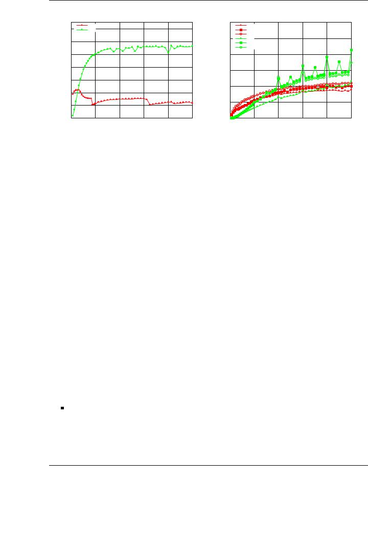
Figure 4.10: Performance of the single-precision unblocked (left) and blocked (right) LU factorization on the multi-core processor and the graphics processor on PECO.

4.5.Computing the LU factorization with partial pivoting on the GPU

4.5.1.Basic implementations. Unblocked and blocked versions

Given the unblocked and blocked formulations of the LU factorization with partial pivoting in Figure 4.9, the procedure followed to implement and evaluate the multi-core and GPU implementation is equivalent to that used for the Cholesky factorization.

Basic scalar and blocked implementations corresponding to the di erent algorithmic variants in Figure 4.9 have been implemented and evaluated on the multi-core CPU and the graphics processor. In these implementations, the information related to pivoting is kept in an integer vector IPIV stored in main memory (also for the GPU implementations). This vector, of dimension n for an (n × n) coe cient matrix, maintains the pivot indices used in the factorization process: for each position i of the vector, row i of the matrix was interchanged with row IPIV(i).

On the GPU, the row interchanges due to the pivoting scheme are performed using the BLAS-1 CUBLASSSWAP routine, that swaps two rows of a matrix stored on GPU memory. Given the high bandwidth delivered by the GPU memory, a lower penalty can be expected from these interchanges than is expected if the interchange occurs in main memory.

The plots in Figure 4.10 report the performance attained for the LU with partial pivoting implementations using the scalar (left-hand plot) and blocked (right-hand plot) algorithmic variants from Figure 4.9. Data transfers are not included in the time measurements, and performance is shown for the optimal block size in the blocked results.

A number of conclusions for the LU implementations which are similar to those extracted for the Cholesky factorization:

The scalar implementations are only convenient on the CPU for relatively small matrix dimensions (up to n = 1,024 in the evaluated algorithmic variant). For these matrix dimensions, the cache system in the multi-core processor plays a critical role on the final attained performance. As in the Cholesky factorization, this motivates the derivation and development of blocked versions of the variants that make use of the advanced memory hierarchy of the multi-cores and the stream-oriented nature of the GPU.

98

4.5. COMPUTING THE LU FACTORIZATION WITH PARTIAL PIVOTING ON THE GPU

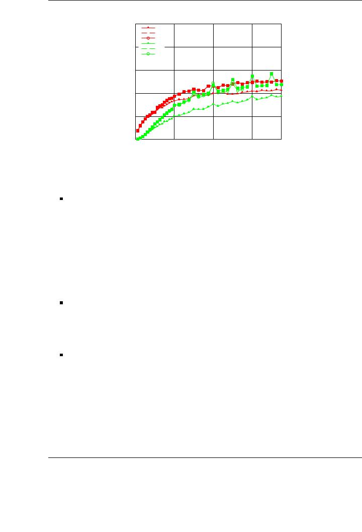
Figure 4.11: Performance of the double-precision blocked LU factorization on the multi-core and the graphics processor on PECO.

The performance rates attained by the blocked implementations are closer to the peak performances of the architectures (107 GFLOPS for the multi-core and 211 GFLOPS for the GPU). These rates illustrate the appeal of blocked algorithms on both types of processors.

As in the Cholesky factorization, the LU factorization on the GPU presents an irregular behavior, with performance peaks for selected matrix sizes, which can be solved by applying the appropriate padding.

In addition, multi-core variants deliver higher performance for small to moderately-sized coe cient matrices. For the tested dimensions, GPU attains higher performance only for matrices bigger than n = 8,000. This also motivates the use of a hybrid approach, mixing the capabilities of each processor for each operation inside the factorization.

In the blocked variants, the derivation and systematic evaluation of all available algorithmic variants (together with the appropriate selection of the block size for each one) makes the di erence between an algorithmic variant that attains lower performance than that of the CPU (see, for example, Variant 1 in Figure 4.10) and another one attaining remarkable speedups (see, for example, Variants 2 and 3 in the figure).

The weakness of the graphics processor when operating with double precision is also revealed in the LU factorization with partial pivoting. Figure 4.11 shows the performance results of the three algorithmic variants developed for the LU factorization, using double precision, on the multi-core platform and the graphics processors. In fact, the GPU implementations barely attain better results than the equivalent multi-core implementations for selected large matrix dimensions, and this improvement is not remarkable. For small/medium matrix sizes (up to n = 8,000), the multi-core architecture outperforms the GPU. This observation is similar to that for the Cholesky factorization, and motivates the usage of mixed-precision techniques, such as the iterative refinement presented in Section 4.6, to overcome this limitation of the GPUs while preserving the accuracy of the solution.

99

CHAPTER 4. LAPACK-LEVEL ROUTINES ON SINGLE-GPU ARCHITECTURES

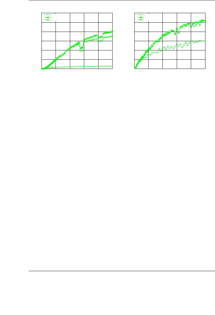
Figure 4.12: Performance of the single-precision blocked LU factorization with padding (left) and hybrid approach (right) on the graphics processor on PECO.

4.5.2.Padding and hybrid algorithm

Regarding matrix dimensions, two main conclusions can be obtained from the evaluation of the algorithmic variants derived for the LU factorization with partial pivoting. First, the irregular behavior of the routines depending on the specific matrix size. Second, the di erent skills of multi-cores and GPUs when factorizing small and large matrices. While the former architectures are especially e cient with matrices of small dimension, GPUs demonstrate their strength in the factorization of larger matrices.

As in the Cholesky factorization, padding and hybrid algorithms are the solutions proposed to solve these two issues, respectively.

Figure 4.12 (left) shows the performance of the three algorithmic variants developed for the LU factorization with partial pivoting on the GPU, applying the appropriate padding to the coe cient matrix. The experimental setup is identical to that used for the basic blocked implementation. Although the peak performance attained for the padded version of the algorithms is similar to that without padding, performance results are more homogeneous, without the presence of peaks in the performance curves shown in the plots.

A similar hybrid approach to that applied for the Cholesky factorization has been applied in the LU factorization with partial pivoting. In this case, at each iteration of the factorization process,

or blocked multi-threaded implementation; and then it is transferred back to the GPU, where the factorization continues.

Figure 4.12 (right) shows the performance of the three algorithmic variants using the hybrid approach. All hybrid variants improve their performance with respect to the corresponding GPUonly implementation. As an example, the peak performance of Variant 2 is increased from 211 GFLOPS to 259 GFLOPS by the hybrid approach.

4.6.Iterative refinement for the solution of linear systems

Graphics processors typically deliver single-precision arithmetic much faster than that of their double-precision counterparts. In previous chapters, significant di erences between singleand

100

4.6. ITERATIVE REFINEMENT FOR THE SOLUTION OF LINEAR SYSTEMS

double-precision performance have been observed for the BLAS-3 routines; in previous sections of this chapter, similar conclusions have been derived from the Cholesky and LU factorizations. The demands that graphical applications set on data precision ultimately determine this behavior, as no double-precision support is usually needed for these applications. In addition, these needs will not likely change in future hardware and software generations. This gap between singleand doubleprecision performance does not only appear in graphical architectures. The Cell B.E. processor announces a theoretical peak performance of 204.8 GFLOPS in single-precision, reducing it to 20 GFLOPS when operating on double-precision data. For general-purpose processors, such as the Intel x87, the use of SSE units can boost performance by doing 4 single-precision flops per cycle, while this rate is reduced to 2 double-precision flops per cycle provided the SSE (or equivalent) extensions are supported by the processor.

However, double precision often the norm in scientific computing in general, and in linear algebra in particular. To solve the performance gap between single and double precision in modern graphics processors, a mixed-precision iterative refinement approach is proposed and evaluated in this section.

In the context of the solution of linear equations, iterative refinement techniques have been successfully applied for many years [104, 93]. Our mixed-precision iterative refinement process combines the benefits of using the GPU to boost single-precision routines with the accuracy of a full double-precision approach.

As a driving example, consider the solution of the linear system Ax = b using Gaussian elimination with partial pivoting, where the coe cient matrix is factored as P A = LU, with L lower triangular, U upper triangular, and P the permutation matrix that results from the factorization. The idea that underlies the iterative process for the accurate solution of a dense linear equation system involves an iterative algorithm with four main steps:

Compute r = b − Ax

Solve Ly = P r

(4.5)

Solve Uz = y Update x′ = x + z

In a mixed precision iterative refinement process, the factorization and triangular solves are carried out using single precision, and only the calculation of the residual and the update of the solution is performed using double precision. Thus, most of the flops involved in the process are carried out in single precision. Naturally, these procedures (especially the factorization, that entails the major part of the calculations) are clear candidates to be executed on the GPU.

This approach has been successfully applied to modern hardware accelerators, such as the Cell B.E. [91]. As a novelty, we propose and evaluate a similar implementation on modern graphics processors that exploits the single precision capabilities of the GPU.

The impact of this approach is that the major part of the operations (factorization of the coe cient matrix and forward/backward substitutions) are performed in single precision, while only the residual calculation and update of the solution are performed in double precision. The striking advantadge is that the final accuracy of the solution will remain the same as that of a full double-precision approach, while the performance of the implementation will benefit from the high performance of the GPU in single-precision computations. The only drawback is the memory needs of the algorithm, as a (single-precision) copy of A must be explicitly stored to calculate the residual at each iteration.

101

CHAPTER 4. LAPACK-LEVEL ROUTINES ON SINGLE-GPU ARCHITECTURES

In our solution, the factorization of matrix A is first computed on the GPU (in single precision arithmetic) using any of the algorithms proposed in the previous sections. Depending on the numerical properties and structure of the coe cient matrix, the Cholesky or the LU factorization with partial pivoting can be used. A first solution is then computed and iteratively refined on the CPU to double precision accuracy.

Algorithm 1 lists the steps necessary to perform the factorization, solution and iterative refinement to solve a dense linear system Ax = b. In this algorithm, the ‘‘(32)’’ subscript indicates single precision storage, while the absence of subscript implies double precision format. Thus, only the matrix-vector product Ax is performed in double precision (BLAS routine GEMV), at a cost of O(n2) flops (floating-point arithmetic operations), while the rest of the non-negligible arithmetic operations involve only single precision operands. The Cholesky factorization is computed on the GPU. A similar strategy can be applied to general systems using the LU factorization.

Our implementation of the iterative refinement algorithm iterates until the solution, x(i+1), satisfies the following condition:

kr(i)k √ kx(i+1)k < ε,

where r(i) is the current residual and x(i) is the current solution, both with a double precision representation, and ε corresponds to the machine (double) precision of the platform. When this condition is satisfied, the algorithm iterates two more steps, and the solution is then considered to be accurate enough [38].

Algorithm 1 Iterative refinement using the Cholesky factorization

A(32), b(32) ← A, b

L(32) ← GPU CHOL BLK(A(32)) x(1)(32) ← L−(32)T (L−(32)1 b(32))

x(1) ← x(1)(32)

i ← 0 repeat

i ← i + 1

r(i) ← b − A · x(i)

r(32)(i) ← r(i)

z(32)(i) ← L−(32)T (L−(32)1 r(32)(i) ) z(i) ← z(32)(i)

x(i+1) ← x(i) + z(i)

until kr(i)k < √ε

kx(i+1)k

Figure 4.13 summarizes the performance results attained for the solution of a linear system Ax = b using our iterative refinement approach. The x axis of the plots represents the dimension of the coe cient matrix; the y axis represents the computation time, in seconds. The times on the left-hand side plot correspond to the case when A is symmetric definite positive, and thus the Cholesky factorization is used to decompose it. On the right-hand side plot, the LU factorization with partial pivoting is used to decompose the coe cient matrix. In both cases, the dark red area corresponds to the factorization time using single precision on the GPU, while the light red area corresponds to the iterative refinement time. The lines in the plots represent the computation time for a full double-precision approach, performing the factorization on the GPU (red line) or on the

102

4.6. ITERATIVE REFINEMENT FOR THE SOLUTION OF LINEAR SYSTEMS

Figure 4.13: Time devoted to factorization and solution of a linear system using double precision on the CPU and the GPU, single precision on the GPU and an iterative refinement strategy on PECO. The Cholesky factorization (left) and the LU factorization (right) are employed to decompose the system matrix.

Table 4.2: Time devoted to factorization and iterative refinement using Cholesky and LU factorizations, and number of iterations necessary to regain full accuracy

CPU (blue line). In this experiment, the iterative refinement is performed exclusively on the CPU; thus, only the factorization of A is performed in the GPU using single precision.

As a first conclusion, the mixed precision approach with iterative refinement presents a remarkable performance gain compared with the double precision factorization and solution on the CPU or the GPU. Our approach permits using the GPU as the platform for the factorization, improving performance while maintaining the accuracy of the solution. If the GPU is only used for the factorization (see red line in the plots), it is not competitive compared with the CPU. With independence of the factorization routine, the time devoted to the iterative refinement process is smaller than that required for the factorization using single precision. Table 4.2 shows a breakdown of the time devoted to the factorization using the GPU and single precision, and the iterative refinement process. In addition, we include the number of iterations required for convergence. As shown, this number is typically small (between 4 and 6 iterations, depending on the matrix size and the factorization routine). For a theoretical study of the upper bound in the number of iterations necessary for convergence, see [123].

The iterative refinement of the solution of a linear equation system represents a trade-o between the high performance of current GPUs operating in single precision and the accuracy delivered by double-precision arithmetic.

103