5.2. LINEAR ALGEBRA COMPUTATION ON MULTI-GPU SYSTEMS

PCI-Express bus

Core0 Core1 Core2 Core3

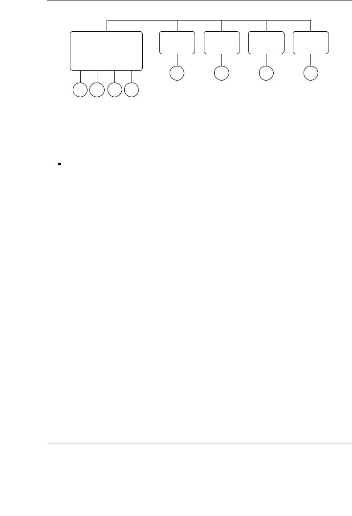
Figure 5.1: Schematic architecture of a multi-GPU system. Each GPU operates with data stored in its own private memory. Communication between GPUs is performed through main memory. Memory spaces are di erent for each GPU in the system, and for the main memory.

Performance: Even with the programmer in charge of data transfers, some decisions to reduce the amount of transfers are hard to take at development/compilation time, and can only be optimized at runtime.

The developed runtime is in charge of managing data dependencies, task scheduling and the general parallelization of the sequential codes, and also of the management of data transfers. Proceeding in this manner, the runtime is responsible of maintaining data coherence among the di erent memory spaces, and applying e ective techniques to reduce the impact of data transfers on the overall parallel performance. This approach completely abstracts the user from the underlying architecture, and thus the existence of separate memory spaces is fully hidden to the developer and transparent to the codes.

5.2.Linear algebra computation on multi-GPU systems

In this section, we introduce some key concepts that, when used in combination, drive to a natural and e cient adaptation of existing linear algebra codes to multi-GPU systems. These concepts include known techniques such as storage-by-blocks and algorithms-by-blocks, that naturally map algorithms to systems that exploit task-level parallelism. Dynamic scheduling and out-of-order execution are key techniques inherited from the superscalar processors that are now reintroduced in software as a way of automatically parallelizing sequential algorithms-by-blocks on novel architectures. Finally, the key concerns taken into account in the design and implementation of the run-time system, together with the key di erences with existing systems are exposed and justified.

5.2.1.Storage-by-blocks and algorithms-by-blocks

Storage of matrices by blocks, where sub-matrices are physically stored and referenced in a hierarchical fashion, presents a few important advantages: a better exploitation of data locality [121], and thus better use of the memory hierarchy in modern architectures, and a more compact storage of matrices with a special structure [8].

From the algorithmic perspective, previous works have advocated for a new alternative to blocked algorithms and storage-by-columns proposed in LAPACK. This alternative, known as

123

CHAPTER 5. MATRIX COMPUTATIONS ON MULTI-GPU SYSTEMS

Figure 5.2: FLASH implementation of the algorithm-by-blocks for Variant 1 of the Cholesky factorization (left) and FLASH implementation of the function FLASH Trsm involved in the algorithm (right).

algorithms-by-blocks [61], considers matrices as a hierarchical collection of sub-matrices, and thus those algorithms operate exclusively with these sub-matrices.

Although one of the main motivations for this class of algorithm-by-blocks is to increase performance [5, 77], this approach can also be used to design and implement runtime systems that exploit tasks parallelism on multi-core architectures and, in our case, on multi-GPU systems. The usage of storage-by-blocks and algorithms-by-blocks eases the task dependency analysis between tasks, and thus allows the development of e cient scheduling techniques to improve parallel performance on this type of architectures.

In response to the increasing interest in algorithms-by-blocks, the FLAME project introduced the FLASH API [95], facilitating the design, implementation and manipulation of matrices stored by blocks. As nearly all linear algebra operations can be expressed using the FLAME notation [29], the conversion of existing algorithms to algorithms-by-blocks is straightforward using the hierarchical matrices provided by the API.

To illustrate this point, Figure 5.2 (left) shows the implementation of the blocked algorithm for the Cholesky factorization using the FLASH API. This implementation is very similar to the corresponding one using the FLAME/C API. The main di erence between both is in the repartitioning FLA Repart 2x2 to 3x3: in FLAME/C, the size of A11 is b × b (thus, it contains b2 scalar elements), while in FLASH this block is of size 1 × 1, as it is considered as one element of a matrix of matrices.

In this type of implementations, routines FLASH Trsm and FLASH Syrk implement the algorithms- by-blocks in Figures 5.2 (right) and 5.3.

124

5.2. LINEAR ALGEBRA COMPUTATION ON MULTI-GPU SYSTEMS

Figure 5.3: FLASH implementation of the function FLASH Syrk involved in the algorithm-by- blocks for Variant 1 of the Cholesky factorization.

125

CHAPTER 5. MATRIX COMPUTATIONS ON MULTI-GPU SYSTEMS

The algorithm-by-blocks for Variant 1 of the Cholesky factorization is next described using an example for a matrix composed by 4 × 4 sub-matrices:

¯

where we assume that each block Aij is of dimension b × b.

The loop in routine FLASH Chol by blocks var1 will iterate four times and, at the beginning of each iteration, the partitioning will contain the following blocks:

Thus, the operations performed on the blocks of the matrix during the first iteration of the loop will be:

The expression in (5.2) operates on a panel of blocks; correspondingly, in routine FLASH Trsm (Figure 5.2-right) the basic operations are also performed on blocks, and thus it is considered an algorithm-by-blocks. When this routine is used to solve the triangular system in (5.2) B := BL−T, three iterations of the loop are performed:

126

5.2. LINEAR ALGEBRA COMPUTATION ON MULTI-GPU SYSTEMS

Thus, the following subroutine calls and matrix operations are performed in those iterations:

Analogously, as the rank-b update in (5.3) involves a blocked sub-matrix, the algorithms-by-blocks in Figure 5.3 provide the necessary functionality.

Similar transformations of the algorithms can be obtained for other variants of the Cholesky factorization, and also for other linear algebra operations. Note the di erences between the algorithm- by-blocks for the Cholesky factorization in Figure 5.2 and the blocked algorithmic variants shown in Chapter 4. First, blocked algorithms assume a classical storage of data by columns, whereas algorithms-by-blocks deal with hierarchical matrices stored by blocks. In addition, while algorithms- by-blocks are decomposed into BLAS calls operating with blocks of the same dimension, blocked algorithms are transformed into BLAS calls with sub-matrices of arbitrary dimensions, yielding operations with di erent matrix shapes (see, for example, the matrix-matrix, panel-matrix or panelpanel blocked algorithms derived for our own implementation of the BLAS routines in Chapter 3).

5.2.2.Dynamic scheduling and out-of-order execution

The development of algorithms-by-blocks naturally facilitates the adoption of techniques akin to dynamic scheduling and out-of-order execution hardwired in superscalar processors. In this section we show how these techniques can be adopted to systematically expose task parallelism in algorithms-by-blocks, which is the base for our automatic parallelization of linear algebra codes on multi-GPU platforms.

Current superscalar processors can dynamically schedule scalar instructions to execution units as operands become available (keeping track of data dependencies). A similar approach can be adopted in software to automatically expose the necessary task parallelism, so that ready tasks are dynamically scheduled available tasks to the available execution resources. The only information that is needed is that necessary to track data dependencies between tasks. In this case, the specific blocks that act as operands of each task, and the directionality of those operands (input for read-only operands, output for write-only operands, or input/output for read-write operands).

Obtaining this information, it is possible to build a software system that acts like Tomasulo’s algorithm [130] does on superscalar processors, dynamically scheduling operations to idle computing resources as operands become available, and tasks become ready for execution.

For example, consider the following partition of a symmetric definite positive matrix to be decomposed using the Cholesky factorization:

Table 5.1 shows the operations (or tasks) that are necessary to factorize A using the algorithm in Figure 5.2. Initially, the original blocks that act as operands to the tasks are available for the corresponding tasks that make use of them. The availability of an operand is indicated in the table using a check tag (2). Upon completion of a task, its output operand is checked in the subsequent entries in the table until that operand appears again as an output variable for another task.

Whenever all the operands of a given task are checked as available, the task can be considered as ready, and thus it can be scheduled for execution. Note how, depending on the order in which

127

CHAPTER 5. MATRIX COMPUTATIONS ON MULTI-GPU SYSTEMS

Table 5.1: An illustration of the availability of operands for each task involved in the Cholesky factorization of a 3 × 3 matrix of blocks using the algorithm-by-blocks shown in Figure 5.2. A 2 indicates that the operand is available. Note how the execution of a task triggers the availability of new subsequent tasks.

128

5.2. LINEAR ALGEBRA COMPUTATION ON MULTI-GPU SYSTEMS

ready tasks are scheduled for execution, the order in which future tasks are marked as ready and scheduled for execution can vary. Therefore, the actual order in which instructions are scheduled and executed does not have to match the sequential order in which tasks are found in the algorithm and added to the table. Consider, e.g., the first three tasks listed in Table 5.1. Initially, tasks 1, 2, and 3 have one of their operands available (A00, A10 and A20, respectively). Task 1 has all operands available, so it can proceed. Tasks 2 and 3, on the other hand, do not have all operands available. After factorizing the first diagonal block (task 1, that updates block A00) the operand A00 marked as input for tasks 2 and 3 becomes available. At that moment, both tasks become ready, as all operands involved are available. The specific order in which those two tasks are scheduled for execution will not a ect the correctness of the computation, but ultimately will influence the order in which future tasks are performed.

In addition to the out-of-order execution, this approach exposes parallelism at a task level (usually referred as task-level parallelism [67]). Following with the example above, after the execution of task 1, both tasks 2 and 3 become ready. As they are independent (that is, there is no data dependency between both tasks) given a system with a pool of execution resources, it is possible to schedule each task to a di erent execution unit such that both tasks are executed in parallel.

It is important to realize that the tasks to perform a given algorithm-by-blocks together with their associated input and output operand identification can be identified a priori, and a table similar to that shown in Figure 5.1 can be systematically built regardless the type of algorithm exposed.

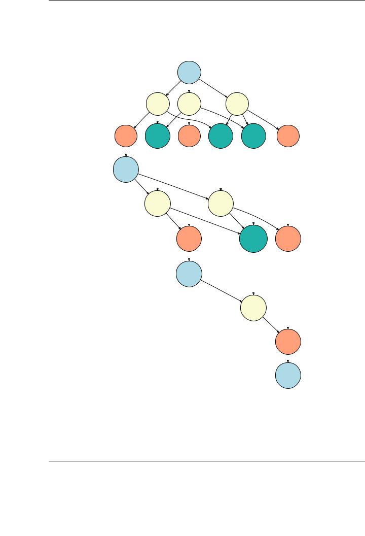
Typically, the information gathered in the table can be represented as a directed acyclic graph (or DAG), in which nodes denote tasks, and edges denote data dependencies between them. For example, Figure 5.4 shows the DAG generated for the Cholesky factorization of a matrix of 4 × 4 blocks. The first two levels of the graph in Figure 5.4 o er a global view of two di erent key aspects of parallelism:

1.Consider the dependence relationship between tasks CHOL0 and TRSM1, where CHOL0 performs the operation A00 := CHOL(A00) and TRSM1 performs the operation A10 := A10A−00T . Note how block A00 is written by task CHOL0 and read by subsequent task TRSM1. Thus, task

TRSM1 cannot proceed until the execution of task CHOL0 is completed, and thus there is a data dependence between them. This type of data dependence, usually referred as flowdependence determines the order in which tasks can be issued to execution.

2.Consider tasks TRSM1, TRSM2, and TRSM3. They are blocked as they are not ready for execution until the execution of task CHOL0 is completed. When block A00 is updated by task CHOL0, all these tasks become ready, and, as there is no data dependency between them, they can proceed concurrently. In this sense, it is possible to execute them in parallel provided there exist enough execution units available. Proceeding this way, a task is seen as the minimum execution unit, and parallelism is extracted at the task level. Thus, task-level parallelism is extracted from the structure of the DAG.

Following these two observations, parallelism can be extracted in algorithms-by-blocks at the task level, with an order of execution ultimately defined by the availability of data operands: this execution model is usually referred as a data-flow execution. These two concepts have been previously applied to multi-core systems [46, 109].

Our main contribution is to redesign this approach to automatically parallelize high-performance dense linear algebra codes on platforms based on multi-GPU architectures with no impact on the libraries already developed for single-GPU systems. This implementation introduces a significant di erence from that for a multi-core target, as multi-GPU systems exhibit separate memory address

129

CHAPTER 5. MATRIX COMPUTATIONS ON MULTI-GPU SYSTEMS

CHOL0

CHOL10

CHOL16

TRSM17

SYRK18

CHOL19

Figure 5.4: DAG for the Cholesky factorization of a 4 × 4 blocked matrix.

130

5.2. LINEAR ALGEBRA COMPUTATION ON MULTI-GPU SYSTEMS

spaces for each execution unit. Given that this feature must remain transparent to the programmer, a run-time system must manage not only the data-flow execution and the task-level parallelism extraction, but also an appropriate scheme to deal with data transfers, reducing them as much as possible without the intervention of the programmer in order to minimize their impact on the final performance.

5.2.3.A runtime system for matrix computations on multi-GPU systems

Independently from the target architecture, there are two parts in a run-time system managing data-flow executions, each one related to a di erent code execution stage. The analysis stage, responsible of building the DAG associated with a specific algorithm; and the dispatch stage, responsible of handling data dependencies at runtime, data positioning issues and dispatching of tasks to execution units.

Data-flow execution entails the usage of a software system with two di erent jobs: tracking data-dependencies and issuing tasks to execution units at runtime. On multi-GPU systems, such a run-time system follows a hybrid execution model, in which the CPU is responsible for scheduling tasks to the accelerators while tracking dependencies at runtime, and the accelerators themselves are responsible for the actual computations and can be viewed as mere execution units.

The analysis stage

Our analysis stage follows many of the ideas implemented for multi-core architectures in the SuperMatrix runtime [120] from the FLAME project. During this stage, a single thread performs a symbolic execution of the code. This symbolic execution does not perform any actual operations as found in the code, but adds them to a queue of pending tasks as they are encountered. For the right-looking algorithm-by-blocks for the Cholesky factorization, this queuing is performed inside the calls to FLA Chol unb var1, FLA Trsm, FLA Syrk, and FLA Gemm as they are encountered in routines FLASH Chol by blocks var1, FLASH Trsm and FLASH Syrk, see Figures 5.2 and 5.3.

Proceeding this manner, the actual tasks involved in the algorithm-by-blocks, together with the existing data dependencies between them, are identified before the actual execution commences, and a DAG can be built to make use of it in during the dispatch stage.

The analysis stage is executed sequentially, and it is not overlapped with the dispatch stage. Other similar runtime systems for multi-core and many-core architectures, such as CellSs or SMPSs, interleave the analysis and dispatch stages, executing them concurrently. That is, the execution of tasks starts as soon as one task is stored in the pending tasks queue. Proceeding this way, the DAG is dynamically constructed, and tasks are issued from the pending queue following a producer-consumer paradigm. Under certain circumstances, this approach has remarkable benefits; for example, if the amount of memory necessary to store the information for the tasks becomes a real bottleneck (due to the limited amount of memory of the platform), the benefit of consuming tasks before the queue is completely built is evident.

However, given that the analysis stage does not perform actual computations, the cost of the symbolic execution stage of dense linear algebra operations is in general amortized during the dispatch stage, so we advocate for a separate execution of both stages. Also, the amount of memory consumed to explicitly store the full DAG can be considered negligible. Therefore, tasks are sequentially stored during the analyzer stage, and the dispatch stage is not invoked until the complete DAG is built.

131