4.3. COMPUTING THE CHOLESKY FACTORIZATION ON THE GPU

without referencing any entry of the upper part of A. In the blocked variants, the algorithm chosen to factorize the diagonal blocks can be the blocked algorithm itself (i.e., a recursive formulation) with a smaller block size, or any scalar algorithm. The latter option is the one illustrated in the figure.

The computational cost of all the algorithmic variants is the same (n3/3 flops); the only difference are the specific BLAS kernels called from each algorithm, and the order in which they are invoked.

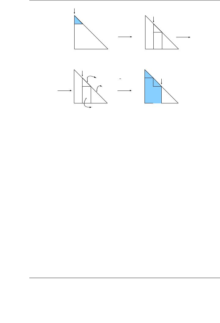
Consider for example the first variant of the blocked algorithm for the Cholesky factorization, and note how the algorithms illustrate, in an intuitive way, the operations that are carried out. Initially, A is partitioned into four di erent blocks, AT L, AT R, ABL and ABR, where the first three are empty (their sizes are 0 × 0, 0 × n and n × 0, respectively). Thus, at the beginning of the first iteration of the algorithm, ABR contains the whole matrix A.

At each iteration of the algorithm, ABR is repartitioned into four new blocks, namely A11, A21, A12 and A22. The elements of the Cholesky factor L corresponding to the first two blocks (A11 and A21) are calculated in the current iteration, and then A22 is updated. The operations that are carried out to compute the elements of the lower triangle of L11 and the whole contents of L21 with the corresponding elements of the Cholesky factor L constitute the main loop of the algorithm:

To the right of the mathematical operations, we indicate the corresponding BLAS-3 routines that are invoked from the blocked algorithms in Figure 4.1. Function TRIL (·) returns the lower triangular part of the matrix passed as a parameter. Thus, the operation A21 := A21TRIL (A11)−T stands for the solution of a triangular system (TRSM routine from BLAS).

Upon completion of the current iteration, the boundaries are shifted, restoring the initial 2 × 2 partitioning, so that ABR is now composed by the elements that were part of A22 at the beginning of the iteration. Proceeding in this manner, in the following iteration the operations on the matrix are applied again on the new block ABR.

The algorithm terminates when ABR remains empty, that is, when the number of rows/columns of AT L equals the number of rows/columns of the original matrix A. The main loop in the algorithm iterates while m(AT L) < m(A), where m(·) corresponds to the number of rows of a given matrix.

4.3.Computing the Cholesky factorization on the GPU

The FLAME algorithms presented in Figure 4.1 for the scalar and blocked Cholesky factorization capture the algorithmic essence of the operations to be implemented. This approach allows an easy translation of the algorithms into high-performance code written in traditional programming languages, like Fortran or C, by just manipulating the pointers to sub-matrices in the partitioning and repartitioning routines, and linking to high-performance parallel BLAS implementations. The FLAME project provides a specific API (FLAME/C) to facilitate the transition from FLAME algorithms to the corresponding C code. This approach hides the error-prone intricate indexing details and eliminates the major part of the debugging e ort when programming linear algebra routines.

The main drawbacks of starting the development process of complex linear algebra libraries (such as LAPACK) on novel architectures from a low level approach are the same as for simpler libraries, such as BLAS. Many key parameters with a dramatic impact on the final performance

81

CHAPTER 4. LAPACK-LEVEL ROUTINES ON SINGLE-GPU ARCHITECTURES

Figure 4.2: Diagram of the blocked Cholesky factorization algorithm, Variant 1.

(scalar and blocked implementations, block sizes on the latter, algorithmic variants, . . . ) can be evaluated more easily at a higher level of abstraction. These observations can be then applied to low level programming paradigms if desired, accelerating the development process of high performance native libraries.

In this section, a number of basic implementations for the scalar and blocked algorithmic variants for the Cholesky factorization presented in previous sections are exposed and their performance evaluated on modern multi-core and graphics processors. A systematic experimental analysis of the optimal algorithmic variants and block sizes is presented. From this basic implementations, successive optimizations, together with the benefits from the performance perspective are reported.

4.3.1.Basic implementations. Unblocked and blocked versions

The FLAME algorithms for the Cholesky factorization present three common stages at each iteration. First, an initial partitioning of the matrices. Second, invocations to the corresponding BLAS routines depending on the specific algorithmic variant. Third, a repartitioning process in preparation for the next iteration. Figure 4.2 illustrates the operations performed at each iteration of the blocked Cholesky algorithm, using Variant 1 from Figure 4.1.

Provided there exists an optimized BLAS implementation, parallel implementations of the Cholesky factorizations for general-purpose multi-core processors usually translate the first and third stages into movements of pointers to define the sub-matrices at each iteration, and the second stage into invocations to multi-threaded BLAS routines.

This approach can be also followed to use the GPU as the target architecture. In this case, the movements of pointers involve memory addresses in the GPU memory, and the invocations to BLAS routines use the NVIDIA CUBLAS implementation. As the NVIDIA CUBLAS routines operate exclusively with matrices previously allocated in the GPU memory, data has to be transferred

82

4.3. COMPUTING THE CHOLESKY FACTORIZATION ON THE GPU

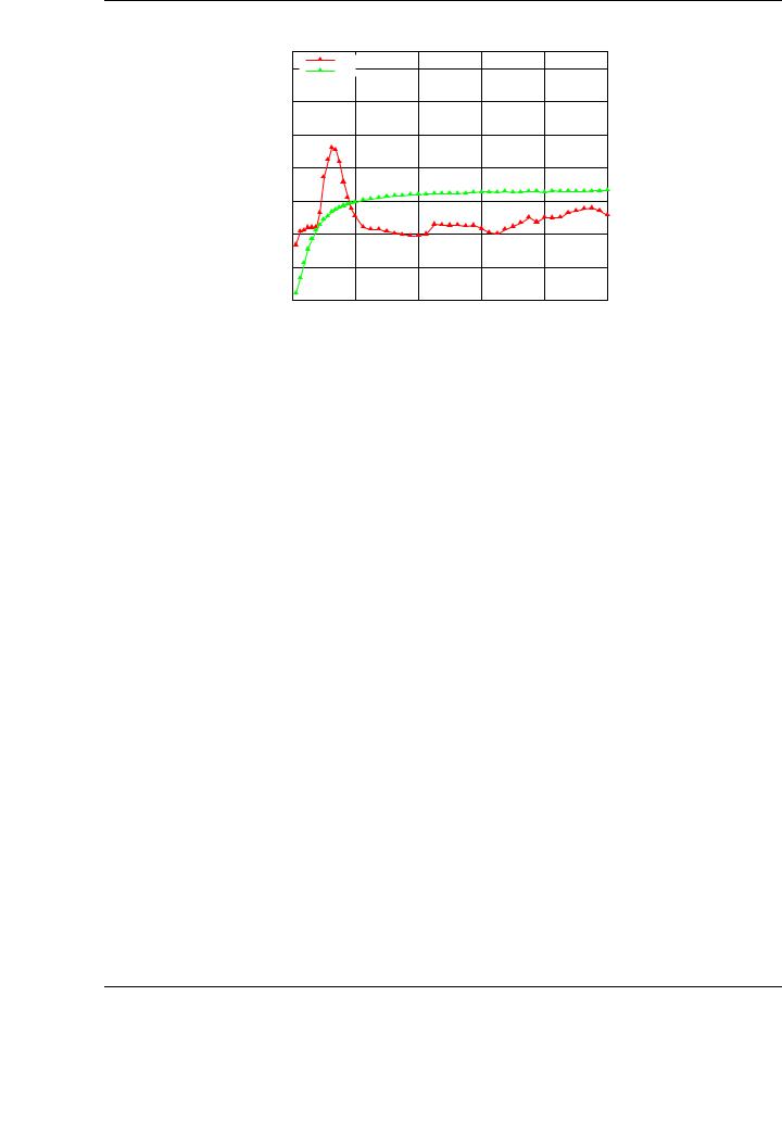
Figure 4.3: Performance of the single-precision scalar variant 1 of the Cholesky factorization on the multi-core processor and the graphics processor on PECO.

before the invocation to the CUBLAS kernels. In our implementations, the whole matrix to be decomposed is initially transferred to the GPU memory. The decomposition is then performed exclusively on the GPU; and the resulting factor is transferred back to main memory.

In order to provide initial implementations of the scalar and blocked algorithms for the Cholesky factorization, the equivalent codes for each algorithmic variant shown in Figure 4.1 have been developed on multi-core and graphics processors.

The scalar versions of the algorithms for the Cholesky algorithmic variants shown in Figure 4.1 imply the usage of BLAS-1 and BLAS-2 routines operating with vectors, and thus they usually deliver a poor performance on recent general-purpose architectures, with sophisticated cache hierarchies. In these type of operations, the access to memory becomes a real bottleneck in the final performance of the implementation. For the scalar algorithms, it is usual that the implementations on multi-cores attain better performance when the matrices to be factorized are small enough to fit in cache memory, reducing the performance as this size is increased and accesses to lower levels in the memory hierarchy are necessary.

To evaluate this impact on multi-core and graphics processors, the first experiment consists on the evaluation of the scalar algorithms presented for the Cholesky factorization. Figure 4.3 reports the performance of the Variant 1 of the scalar algorithm for the Cholesky factorization on a multi-core processor using a tuned multi-threaded BLAS implementation and its equivalent implementation on the GPU using NVIDIA CUBLAS. In the implementation using the graphics processor, only the square root of the diagonal element is performed on the CPU, transferring previously the diagonal element to main memory, and back to GPU memory when the update is done. Experimental evidences [23] revealed the benefits of using the CPU to perform this operation, even with the penalty introduced by the transfer of the scalar value between memory spaces. Performance results are given in terms of GFLOPS for increasing matrix sizes; hereafter, transfer times are not included in the performance results. We have chosen this algorithmic variant as the most illustrative, as the remaining variants o ered worse performance results, but a similar qualitative behavior.

83

CHAPTER 4. LAPACK-LEVEL ROUTINES ON SINGLE-GPU ARCHITECTURES

Figure 4.4: Performance of the single-precision blocked algorithmic variants of the Cholesky factorization on the multi-core processor and the graphics processor on PECO.

The performance rates attained by the scalar implementations, is far from the peak performance of the architecture for both the CPU and the GPU, and also very di erent from the performances attained for the BLAS-3 routines studied in Chapter 3. More specifically, the performances obtained in this case are 9.2 GFLOPS and 6.5 GFLOPS for the CPU and the GPU, respectively. These results represent a small percentage of the peak performance of the architectures. Considering the performance of the GEMM implementation as a realistic peak performance of both architectures (see Figure 3.1), the results obtained for the scalar Cholesky implementations are roughly a 7% of that maximum GFLOPS rate on the CPU and a 2% for the GPU.

As these kernels are part of the blocked variants (the factorization of the diagonal blocks is usually performed by invoking scalar variants of the factorization routines), it is important to analyze its performance. The cache memories in the general-purpose processors play a critical role for BLAS-1 and BLAS-2 operations that usually appear in the scalar variants of the codes. More specifically, they have a direct impact on the performance of the scalar routines for small matrix sizes (up to n = 2,500 in the unblocked Cholesky factorization, for example). For these matrix sizes, the use of the CPU o ers important speedups compared with the equivalent implementation on the GPU. For larger matrices, however, the GPU (without a sophisticated memory hierarchy) attains higher performance ratios.

These performance results lead to the conclusion that a blocked version of the algorithms becomes necessary to attain high performance, not only on multi-core processors, but also on modern graphics processors, especially if large matrices are involved in the factorizations. For relatively small matrices, however, the usage of the CPU can be still an appealing option.

The performance of the blocked algorithms for the Cholesky factorization is shown in Figure 4.4. The experimental setup is the same as that used for the evaluation of the scalar algorithms. A full study of the block sizes has been carried out, reporting only the results corresponding to the optimal one in the figures. The figure reports the performance results for the three blocked algorithmic variants, both on the multi-core processor and the graphics processor. In the latter case, the diagonal block is factorized using the corresponding variant of the scalar algorithm.

84

4.3. COMPUTING THE CHOLESKY FACTORIZATION ON THE GPU

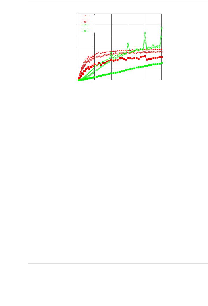
Figure 4.5: Impact of the block size on the single-precision Cholesky factorization using the graphics processor on PECO.

The attained performance for the blocked algorithms, independently from the target processor, is illustrative of the benefits expected for these type of implementations. These rates are closer to those attained for the BLAS-3 routines reported in Chapter 3. In this case, the peak performance obtained for the Cholesky factorization (using Variant 3) is 235 GFLOPS, which means a 65% of the performance achieved by the GEMM implementation in NVIDIA CUBLAS.

A deeper analysis of the performance rates involves a comparison between scalar and blocked implementations, a study of the impact of the block size and algorithmic variants on the final performance results on blocked algorithms and a comparison between single and double precision capabilities of the tested architectures. This analysis is presented progressively and motivates the improvements introduced in the following sections.

Impact of the block size

In the blocked Cholesky implementations, besides the specific algorithmic variant chosen, the block size (b) plays a fundamental role in the final performance of the implementation. In the GPU implementations, the block size ultimately determines the dimensions of the sub-matrices involved in the intermediate steps of the decomposition. As shown in Chapter 3, the implementations of the BLAS on GPUs deliver very di erent performance depending on the size of the operands. Thus, the operands form and size will ultimately determine the final performance of the Cholesky algorithms that make use of them.

Figure 4.5 shows GFLOPS rate of the first algorithmic variant for the blocked Cholesky implementation on the GPU. In the plots, we show the performance attained by the implementation with block size varying from b = 32 to b = 512. The right-hand side plot is a detailed view of the same experiment for a smaller set of matrix dimensions.

Taking as a driving example a coe cient matrix of dimension n = 20,000, performance grows as the block size is increased, reaching an optimal point for b = 128. From this value on, performance decreases, attaining the worst value for the largest block size tested (b = 512). The di erence in performance between both extremes is significant: 204 GFLOPS for b = 512 and 237 GFLOPS for b = 128. This performance di erence (an improvement of 16% between both values of b) gives an idea of the importance of a thorough and systematic evaluation of the block size to find the optimal one, and is a major contribution of our evaluation methodology. Similar behavior has been

85

CHAPTER 4. LAPACK-LEVEL ROUTINES ON SINGLE-GPU ARCHITECTURES

observed in the rest of the algorithmic variants and matrix dimensions. All performance results shown in the rest of the evaluation only show the results for the optimal block size.

Scalar implementations vs. blocked implementations

As previously stated, blocked algorithms are the most convenient approach to the development of dense linear algebra routines such as the Cholesky factorization on modern multiand many-core architectures.

In the target architectures, the scalar implementation of the algorithmic Variant 1 attains 6.5 GFLOPS on the graphics processor and 5.1 GFLOPS on the multi-core processor for the largest tested matrices: see Figure 4.3. In the case of the GPU, this is the best result from the whole set of tested dimensions. On the other hand, in the multi-core processor the role played by cache memory reveals for small matrices, attaining 9.2 GFLOPS for matrices of dimension n = 2,500. The performance of the scalar implementation on the CPU drops rapidly from this dimension on, attaining similar performance results than those attained on the GPU.

On the other hand, taking as a reference the best algorithmic variant for the blocked implementation on each processor, the di erences with respect to the performance attained using the scalar implementations are remarkable, see Figure 4.4. The performance achieved on the GPU is 235 GFLOPS for the largest tested matrix, and 141 GFLOPS in the case of the CPU. The speedup obtained in this basic implementations (1.7× comparing the best blocked algorithmic variant on the CPU and on the GPU) is the base for further optimizations. In this case, the best performance results are attained for the largest tested matrices.

From the comparison between the scalar and the blocked implementations, the first conclusion to be extracted is the convenience of using blocked algorithms for the Cholesky factorization not only on multi-core processors, but also on modern graphics processors. In the latter architecture, the usage of BLAS-3 routines involves operations with higher arithmetic intensity, for which the GPU unleashes its true potential [82].

Performance of the di erent algorithmic variants

The results shown in Figure 4.4 show the capital importance of choosing the appropriate algorithmic variant in the computation of the Cholesky factorization. The specific underlying BLAS calls invoked in each variant (and shown in the algorithms of the Figures 4.1), as well as the specific shape of the involved sub-matrices depends on the algorithmic variant, determine the performance of the corresponding variant.

More specifically, the performance of the GPU implementations vary between 235 GFLOPS for Variant 3 to 77 GFLOPS for Variant 2. The performance attained for Variant 1 is similar to that attained for Variant 3. On the CPU, the attained performance rates are also greatly a ected by the specific algorithmic variants, ranging from 105 GFLOPS to 141 GFLOPS for the worst and best variant, respectively.

Therefore, a systematic derivation of all the algorithmic variants for a given dense linear algebra operation (in this case, the Cholesky factorization) becomes absolutely necessary to find out the optimal one. The use of the high-level approach followed in our methodology eases this systematic derivation process. Moreover, the optimal variants on the GPU di er from those on the CPU, and are likely to be also di erent for other GPU models, BLAS implementation or accelerator type. This justifies the detailed development and evaluation of several algorithmic variants, together with its careful evaluation. The adopted high-level approach allows the library developer to extract critical

86

4.3. COMPUTING THE CHOLESKY FACTORIZATION ON THE GPU

Figure 4.6: Performance of the double-precision blocked algorithmic variants of the Cholesky factorization on the multi-core processor and the graphics processor on PECO.

insights about the final performance of the implementations without having to develop low-level codes.

Single/double precision capabilities of the GPU

Figure 4.6 reports the performance rates for the three algorithmic variants of the Cholesky factorization on the multi-core processor and the GPU, using double precision. The experimental setup used for the test is identical to that used for single precision.

The comparison between the performances of the single and double precision implementations of each variant of the Cholesky factorization reports the capabilities of each type of processor depending on the arithmetic precision. Both processors experiment a reduction in the performance when operating with double precision data. However, this reduction is less important for the general-purpose processor: 50% of the performance attained for single precision arithmetic. The drop is dramatically higher in the case of the GPU: double-precision performs at 25% of the pace attained for single-precision arithmetic. Peak performances are 53 GFLOPS on the GPU, and 68 GFLOPS on the CPU. The qualitative behavior of the algorithmic variants is the same as that observed for the single-precision experiments.

A quick conclusion is that (pre-Fermi) GPUs as that evaluated in this chapter are not competitive in double precision for this type of operations. This observation motivates the iterative refinement approach presented in Section 4.6.

Impact of the matrix size in the final performance

The analysis of the performance results attained for the blocked implementations admits two di erent observations:

From a coarse-grained perspective, the performance results attained with single/doubleprecision data (see Figures 4.4/4.6, respectively) show a di erent behavior depending on the target processor type. In general, the performance curves for the CPU implementations

87