3.3. IMPROVEMENTS IN THE PERFORMANCE OF LEVEL-3 NVIDIA CUBLAS

Table 3.4: Di erent names given to the partitioned sub-matrices according to their shapes.

3.3.2.Systematic development and evaluation of algorithmic variants

The GEMM-based approach exploits the usual near-optimal performance of the GEMM routine in many BLAS implementations. In addition to the performance of the specific kernels used in each routine, a second key factor in the final performance achieved for each implementation is the shape of the blocks involved in those inner kernels. For general-purpose architectures, those shapes have a direct impact on important factors such as cache memory exploitation, number of TLB misses or register usage [72], to name only a few.

For a given linear algebra operation, there usually exists a set of loop-based algorithms. The number of flops involved is exactly the same for all algorithmic variant, operating on the same data. The di erence between them is basically the order in which operations are performed and, in blocked algorithms, the performance of the specific underlying BLAS operations.

In our case, the performance of the routines in NVIDIA CUBLAS in general, and that of the GEMM implementation in particular, are considerably influenced by the shape of its operands, as shown in the performance evaluation of Section 3.2.1, Figure 3.4. Thus, it is desirable to have multiple algorithmic variants at the disposal of the library user so that the best algorithm can be chosen for each situation. Even though the operations ultimately performed by each algorithmic variant are the same, there are many factors di cult to predict or control that can be exposed and solved by the di erent algorithmic variants.

Let us illustrate this with an example: the derivation of di erent algorithms for the GEMM operation. Given an m × n matrix X, consider two di erent partitionings of X into blocks of rows and blocks of columns:

where Xj has nb columns and Xi has mb rows. For simplicity, we will assume hereafter that the

number of rows/columns of X is an integer multiple of both mb and nb.

Depending on the dimensions of the sub-matrices (blocks) obtained in the partitioning process, we denote them as matrices, panels or blocks, as detailed in Table 3.4. The implementation of the matrix-matrix multiplication can be decomposed into multiplications with those sub-matrices. Thus, by performing di erent row and column partitioning schemes for the matrices A and B, it is possible to derive three di erent algorithmic variants, depending on the specific shapes of the sub-matrices involved. The name received by each variant depends on the shapes of the operands in them:

Matrix-panel variant (GEMM MP): Figure 3.7 represents an algorithm in which, for each iteration, the computation involves a matrix (A) and a panel of columns (B1), to obtain

59

CHAPTER 3. BLAS ON SINGLE-GPU ARCHITECTURES

a new panel of columns of C. The algorithmic variant that proceeds this way is shown in Figure 3.8.

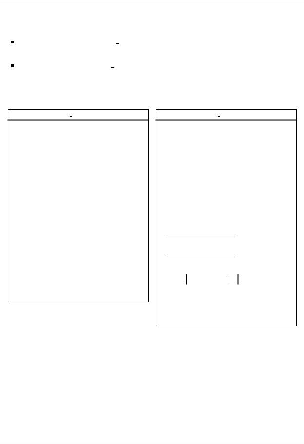
Panel-matrix variant (GEMM PM): In each iteration, a panel of rows of matrix A is multiplied by the whole matrix B, to obtain a new panel of rows of the result matrix C.

Panel-panel variant (GEMM PP): In the each iteration, a panel of columns of matrix A and a panel of rows of matrix B are multiplied to update the whole matrix C.

The algorithms in FLAME notation for the last two variants are shown in Figure 3.10.

Figure 3.10: Algorithms for computing the matrix-matrix product. Panel-matrix variant (left), and panel-panel variant (right).

Several algorithmic variants with matrix-panel, panel-matrix and panel-panel partitionings are also possible for the rest of BLAS-3. To show this, we propose three di erent algorithmic variants for the SYRK operation C := C − AAT (with only the lower triangular part of C being updated), presented in FLAME notation in Figure 3.11. For each iteration of the loop, the algorithms in that figure also include the BLAS-3 kernel that has to be invoked in order to perform the corresponding operation.

60