

Книги по МРТ КТ на английском языке / MR Imaging in White Matter Diseases of the Brain and Spinal Cord - K Sartor Massimo Filippi Nicola De Stefano Vincent Dou
.pdfQuantitative Diffusion Imaging |
63 |
6Quantitative Di usion Imaging
Peter C.M. van Zijl, Lidia Nagae-Poetscher and Susumu Mori
CONTENTS
6.1Introduction 63
6.2Diffusion Basics 64
6.3 |
Diffusion Tensor Imaging (DTI) |
66 |
6.3.1 |
Tensor Properties and Calculations 66 |
|
6.3.2 |
Diffusion Anisotropy Definitions |
67 |
6.4 |
DTI Data Acquisition 68 |
|
6.4.1Trace Imaging 69
6.4.2Anisotropy Imaging 69
6.5 |
Axonal Mapping/Fiber Tracking 71 |
6.6Applications of Quantitative DWI/DTI
to the Brain 72
6.6.1Normal Control Values of Diffusion Parameters
|
During Early Development and Aging |
72 |
6.6.2 |
Diffusion Imaging of Acute Ischemia |
75 |
6.6.3 |
Initial Applications in Other Diseases |
77 |
6.7Conclusions 77 References 78
6.1 Introduction
The basic principles of diffusion magnetic resonance imaging (MRI) were established in the mid 1980s (for recent reviews see Le Bihan 2003; Le Bihan and van Zijl 2002), combining principles of MRI with principles of diffusion sensitization through the use of pairs of magnetic field gradient pulses. The potential of diffusion MRI is based on the notion that, while diffusing, water molecules probe tissue structure at a microscopic scale well beyond the usual image resolution. During typical diffusion periods of about 50–100 ms, water molecules (water is the most convenient molecular species to study with diffusion MRI, but some metabolites may also be studied with
P. C. M. van Zijl
Johns Hopkins University Medical School, Department of Radiology, 217 Traylor Bldg., 720 Rutland Ave., Baltimore, MD 21205, USA
L. Nagae-Poetscher; S. Mori
F. M. Kirby Research Center for Functional Brain Imaging, Kennedy Krieger Institute, 707 N. Broadway, Baltimore, MD 21205, USA
spectroscopy; Moonen et al. 1990; van Zijl et al. 1994) move in the brain on average over distances of around 10–20 ìm, bouncing, crossing, or interacting with many tissue components, such as cell membranes, fibers, or macromolecules. The overall effect observed in a diffusion MRI image volume element (voxel) therefore reflects, on a statistical basis, the displacement distribution of the water molecules present within this voxel. The non-invasive observation of this displacement distribution in vivo thus provides unique clues on the structure and geometric organization of tissues. Since the initial work by Le Bihan, the developments in the application of diffusion imaging and spectroscopy in vivo have been rapid (Table 6.1). The most successful application of diffusion MRI since the early 1990s has been acute brain ischemia (Moseley et al.1990a; van Gelderen et al. 1994; Baird and Warach 1998; Sotak 2002). Brain data show that diffusion is anisotropic in white matter (Moseley et al. 1990b), leading to the opportunity to probe the cumulative effect via so-called trace imaging (van Gelderen et al. 1994; Mori and van Zijl 1995) (or isotropic diffusion imaging) or to develop a formalism to quantify this anisotropy in an orientationally independent manner (Basser et al. 1994a; Basser and Pierpaoli 1996; Basser and
Jones 2002; Pierpaoli and Basser 1996). This latter formalism has provided not only a means to study the magnitude of diffusion anisotropy (Pierpaoli and Basser 1996; Pierpaoli et al. 1996; Ulug and van Zijl 1999), but also the possibility to acquire orientational information from two-dimensional color maps (Pajevic and Pierpaoli 1999) or from threedimensional tracking of major white matter fibers (Mori et al. 1999; Conturo 1999; Jones et al. 1999a; Basser et al. 2000; Poupon et al. 2000; Mori and van Zijl 2002). This development has started a new era of connectivity imaging that is presently making rapid progress.
In this chapter, we will first describe the principles of isotropic and anisotropic diffusion, together with approaches to create image contrast based on these properties. The basics of why it is needed to use a ten-

64 |
|
P. C. M. van Zijl et al. |
Table 6.1. History of some important in vivo diffusion MRI and MRS developmentsa |
|
|
|
|
|
Year |
Advance |
Reference(s) |
|
|
|
1986 |
Le Bihan et al. report first in vivo diffusion images |
Le Bihan et al. (1986) |
1990 |
Moonen et al. report first in vivo diffusion spectroscopy |
Moonen et al. (1990) |
1990 |
Moseley et al. show early ADC changes in acute stroke |
Moseley et al. (1990a) |
1990 |
Moseley et al. show diffusional anisotropy in cat brain |
Moseley et al. (1990b) |
1992 |
Warach et al. first measure stroke patients using DWI |
Warach et al. (1992) |
1994 |
Van Gelderen et al. suggest use of tensor trace to better observe ischemic lesions |
Van Gelderen et al. (1994) |
|
through removal of the diffusion anisotropy |
|
1994 |
Davis et al. show ADC changes within 2–3 min of ischemic onset |
Davis et al. (1994) |
1994 |
Basser et al. introduce theory for diffusion tensor imaging |
Basser et al. (1994a,b) |
1996 |
Basser and Pierpaoli design orientation-independent anisotropy indices |
Pierpaoli et al. (1996); |
|
|
Pierpaoli and Basser (1996) |
1997 |
Makris uses DTI to design fiber color scheme |
Makris et al. (1997) |
1999 |
Mori et al. report successful tracking of white matter fibers; |
Mori et al. (1999); Conturo |
|
Conturo et al. and Jones et al. report first human data |
et al. (1999); Jones et al. (1999) |
1999 |
Jones et al. discuss importance of multi-directional diffusion acquisition |
Jones et al. (1999) |
2000 |
Wiegell et al. report imaging of fiber crossings |
Wiegell et al. (2000) |
aThe above table focuses on medical technology rather than NMR literature and clinical discoveries. Notice that in the 1960s, 1970s and 1980s, much NMR literature appeared on excised tissue diffusion properties and anisotropy determination. This literature is not included here because we focus on in vivo work, but a comprehensive review of this early work is available from Karger et al. (1988).
sor to describe diffusion in tissue will be explained, and schemes to generate orientation-independent diffusion tensor descriptions will be discussed. Subsequently, it will be discussed how to optimally acquire the experimental data needed for the tensor description and how the results will depend on the range of b-values and the number of directions used. This will be followed by a brief overview of recent applications.
6.2
Di usion Basics
Diffusion is defined as a process by which random molecular motion transports matter from one part of a system to another. In an isotropic medium such as neat water, this process can be described by a single coefficient, i.e., the diffusion constant D, and a characteristic equation of motion. This diffusion equation, also known as Fick’s second law, states that the change in the concentration C (or the amount of matter transported) in time is proportional to the change in the concentration gradient with respect to the positional coordinates:
∂C |
= D 2C |
[6.1] |
|
||
∂t |
|
|
in which 2 = δ 2 . The magnitude of diffusion is thus
δ r2
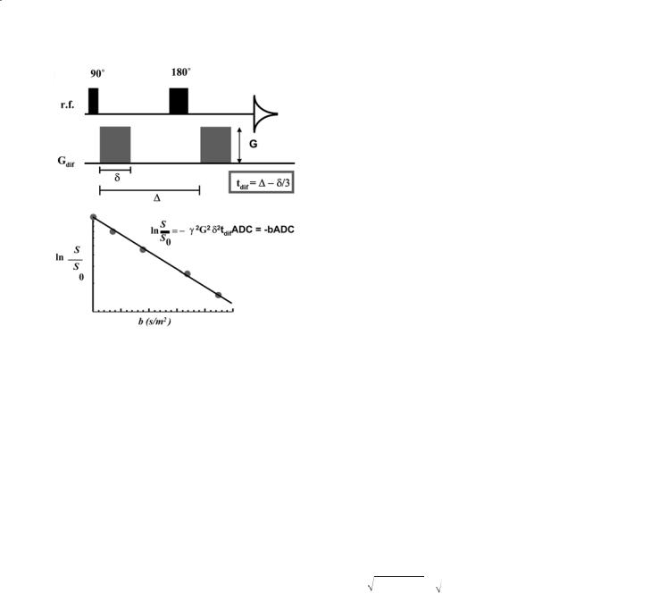
defined as the flux of molecules per time unit (m2/s). MRI can measure diffusion through application of self-refocusing pairs of magnetic field gradients (Fig. 6.1) (Stejskal and Tanner 1965). The random phase loss due to diffusion between different spatial locations can not be refocused and a signal loss is found that will depend on the gradient strength G, gradient length δ, and the time over which diffusion is measured, the diffusion time tdif , which depends both on the time period between the starts of the two diffusion gradients (∆) as well as on their length and shape.For rectangular gradients and free (isotropic) Gaussian diffusion, this is described by the basic Stejskal-Tanner equation:
S / S0 = e−γ 2G2δ 2tdif D = e−γ 2G2δ 2 (∆ −δ /3)D = e−bD |
[6.2] |
The b-value, describing the product of the gradient and timing constants, was introduced by Le Bihan et al. (1986). When combining diffusion weighting with imaging, the results are known as diffusion-weighted imaging (DWI), a term now common in clinical imaging. The DW contrast adds to other contrast in the image, including spin density, T1, and T2 contrast. To obtain pure diffusion information, it is necessary to acquire the diffu- sion-based signal decay as a function of b-value (at least two in an isotropic system), leading to absolute
Quantitative Diffusion Imaging |
65 |
a
b
Fig. 6.1a,b. a Typical spin-echo Stejskal Tanner pulse sequence for diffusion weighting with a pair of pulsed field gradients of strength G and length d. Data acquisition is denoted by a free induction decay. b Calculation of the apparent diffusion constant (ADC) from a linear fit of the normalized logarithmic signal decay as a function of b-factor. The diffusion time and signal decay are defined for a pair of square field gradients
diffusion images, in which the D-value is displayed as a function of space.
When studying biological systems, the environment is in general anisotropic and the imaging volume will reflect a weighted average of multiple compartments with different diffusion constants. This weighting will depend on the size of the compartments, their properties (viscosity, binding with macromolecular structures, etc.), as well as on the barriers between them (exchange). Due to this environmental dependence, it is common to speak of the apparent diffusion coefficient (ADC). This situation provides the opportunity to study tissue microstructure by varying the length of the diffusion time. For instance, under the condition of permeable compartment separations, two extreme situations can be distinguished. For very long diffusion times, water molecules can probe most compartments “i” with populations pi, which can be seen as fast exchange on the measurement time scale:
−b∑ pi Di |
= e−b(ADC) |
|
S / S0 = e i |
[6.3a] |
For very short diffusion times (or very impermeable barriers) water molecules most probably stay
within their compartments and the condition of slow exchange is approached, under which the measured “approximately-exponential” signal decay at low b- values is built up of contributions of the signal decays in individual compartments. Neglecting relaxation contributions, one has:
S / S0 = ∑ pie−bDi e−b(ADC) |
[6.3b] |
i |
|
As a consequence, classical (Gaussian) treatment of the diffusion process may not properly reflect the tissue properties. Interestingly, the practical situation is that, at sufficiently low b-values (< ~1000 s/mm2) and within experimental accuracy, the in vivo situation can generally be described by a single exponential, as used in Eq. 6.3a,b. This simple “single-expo- nential” situation is no longer valid when going to higher b-values as has been demonstrated in cell systems (van Zijl et al. 1991, 1994; Andrasko 1976b), as well as in vivo (for a recent review see Cohen and Assaf 2002). In cell suspensions or perfused cell systems, this situation can generally be approximated by a biexponential description for intraand extracellular diffusion, including the membrane transport if necessary. In tissue, despite the appearance of a biexponential, the situation is probably more complex. Attempts to understand this in vivo behavior are now a hot topic of discussion.
To get an impression of the distance scale measured by diffusion imaging, it is convenient to start with free diffusion, in which the radius of the diffusion sphere is given by the standard deviation of the Gaussian displacement profile.This is reflected by the well-known Einstein equation for the mean square displacement:
σ = rrms = x2 + y2 + z2 = 2Dtdif |
[6.4] |
Free water diffusion at 37˚C corresponds to D=3 × 10⁻⁹ m2/s, which can be taken as an upper limit in vivo and is closely approximated in cerebral spinal fluid (CSF). In tissue, a D-value of about 1.5 × 10- 9 m2/s is a frequent estimate for free cellular diffusion.In a clinical scanner,available gradient strengths limit diffusion times to the order of about 40–50 ms, corresponding to a free diffusion distance of about 12 µm. Cellular restrictions in the brain (membranes, organelles, macromolecules) are found over much smaller distances, and reduced diffusion constants are measured for both gray and white matter. One way to probe the spatial boundaries is by assessing displacement probabilities using so-called q-space imaging (Callaghan et al. 1991, 1999; Cory and

66 |
P. C. M. van Zijl et al. |
Garroway 1990), in which q is the reciprocal spatial vector (units of m–1), defined as (γGδ/2π). Under the conditions of δ<∆, the magnitude of q controls the signal decay via:
S( |
|
)/ S0 = ∫P( |
|
,∆)e(i2π q |
R |
)d |
|
|
q |
R |
R |
[6.5] |
in which R is the average displacement vector and P(R,∆) the displacement probability distribution function. Recent work by Assaf and Cohen (2000) indicates that the slower component (i.e., the one remaining at high b-value) measured from biexponential analysis of the diffusion decay in the brain has a displacement probability of about 2 µm, and concluded that this is probably due to the brain fibers, where restrictions are formed by axonal (~3 µm) and myelin diameters (1–2 µm), leading to orientationally restricted diffusion. However, such orientational restrictions can also be detected using lower b-values (Beaulieu 2002), as has been demonstrated in recent years using diffusion tensor imaging.
6.3
Di usion Tensor Imaging (DTI)
6.3.1
Tensor Properties and Calculations
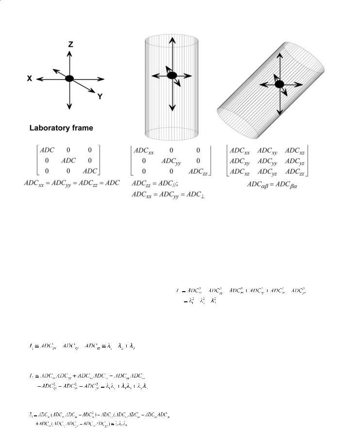
The presence of spatial restrictions in tissue causes water diffusion to be orientationally dependent. This is illustrated in Fig. 6.2. Diffusion is measured in the so-called laboratory frame, defined by the axes of the MRI scanner (z-axis along the field, x and y perpendicular and given by the gradient directions). When diffusion is isotropic (Fig. 6.2a), measurement of diffusion constants using the x, y, or z-gradients will all give the same value. If diffusion is anisotropic, this is no longer the case. For instance, in Fig. 6.2b diffusion is restricted by a cylinder along the z-axis, leading to the measurement of two different diffusion constants (ADC and ADC ). Obviously, in practice, such a situation will not occur and the restrictions will be randomly oriented in the laboratory frame. As a consequence, diffusion is generally described by a tensor (Fig. 6.2c) (van Zijl et al. 1994; van Gelderen et al. 1994; Karger et al. 1988; Basser et al. 1994b). As diffusion constants are real values, this is a symmetric tensor (ADCαβ = ADCβα ; α ≠ β; α, β, {x,y,z}) characterized by six unique diffusion constants. Consequently, the
signal decay is not described by the simple equation [2] above, but rather by:
2 2 |
|
|
|
|
|
|
|
−γ 2δ 2tdif ∑Gα Gβ ADCα β |
− ∑bα β ADCα β |
|
|
|
|
|
|
|
|
||||
S / S0 = e−γ δ |
tdif G D G = e |
α ,β |
= e α ,β |
α, β {x, y, z} |
||||||
[6.6]
.
Thus, at least seven measurements are needed to determine these tensor elements (one at low b-value and six directions at high b-value). This complicates and slows down image analysis. For instance, when trying to identify stroke lesions, anisotropy effects may be very cumbersome and confusing in ischemic regions. As a consequence, the first practical application of diffusion tensor imaging involved the acquisition of a reduced data set, removing the anisotropy information inherent in the tensor and creating an image representing the trace of the tensor at any given point (van Gelderen et al. 1994; Mori and van Zijl
1995), which is a rotationally invariant quantity. This has become especially important in the clinic for detection of ischemic lesions (Baird and Warach 1998; Sotak 2002; Ulug et al. 1997). On the other hand, the analysis of diffusion anisotropy in vivo may provide important new information regarding tissue microstructure. This field was pioneered by Pierpaoli and Basser (1996) and Pierpaoli et al. (1996), who defined orientationally independent anisotropy indices based on intrinsic structural properties of ellipsoids (magnitude, volume, etc.) that can be used to quantify the tissue anisotropy properties in an unbiased manner between subjects.
In order to assess such diffusion anisotropy in an orientation-independent manner, the diffusion tensor (measured in the laboratory frame, as detailed in the next section on data acquisition) needs to be diagonalized to determine the magnitude of the apparent diffusion constants in each voxel. The magnitude of the three resulting ADCs, the eigenvalues γ1,γ2,γ3, determine the shape of the so-called diffusion ellipsoid. The orientation of the ellipsoid in the laboratory frame is determined by the rotation matrix, R, containing the three eigenvectors
. ADCxx |
ADCxy |
ADCxz |
→ R |
λ1 |
0 |
0 |
|
|||||
ADCxy |
ADCyy |
ADCyz |
0 |
λ2 |
0 |
R |
||||||
|
|
|
|
|
|
|
|
diagonalize |
−1 |
|
|
|
ADC |
xz |
ADC |
yz |
ADC |
zz |
|
|
0 |
0 |
λ |
|
|
|
|
|
|
|
|
|
|
3 |
[6.7] |
|||
|
Laboratory frame |
|
|
diagonal frame |
||||||||
After diagonalizing the tensor, the eigenvalues can be used to calculate a multitude of diffusion anisotropy indices. However, there are some potential problems. For most of these indices, the eigenvalues
Quantitative Diffusion Imaging |
|
67 |
a |
b |
c |
Fig. 6.2a–c. a Laboratory frame in a diffusion experiment. The z-axis is along the magnetic field; x,y,z are the gradient directions. For isotropic diffusion (a), all tensor elements are equal. b For diffusion in a tube with cylindrical symmetry oriented along the field, there are two different diffusion constants, namely parallel to the tube and perpendicular. c In vivo, the orientation of fibers or other structures may not be along the field, and the diffusion has to be described by a symmetric tensor with six different elements. Average local geometry can be deduced using a diagonalization procedure
need to be ranked by magnitude, which may introduce a bias in the presence of noise (Pierpaoli and Basser 1996; Pierpaoli et al. 1996). To avoid this,
Pierpaoli et al. (1996) and Pierpaoli and Basser
1996 designed indices that combine tensor elements to represent ellipsoid properties that are invariant with respect to such ordering. These properties are based on three basic invariants of a tensor, which are (Ulug and van Zijl 1999):
structed from the basic three above. A common one is:
Square of tensor magnitude:
[6.8d]
1st invariant (trace):
[6.8a]
2nd invariant:
[6.8b]
3rd invariant (determinant):
[6.8c]
These three invariants are sufficient to completely describe the tensor. Further invariants can be con-
6.3.2
Di usion Anisotropy Definitions
As can be seen from the equations, the invariant properties have units of ADC, ADC2, and ADC3, which relate to the average ADC, the surface, and the volume of the ellipsoid (Ulug and van Zijl 1999). Thus, a set of diffusion constants can be defined describing such inherent properties of the ellipsoid. Alternatively, one can define diffusion anisotropies reflecting such ellipsoid properties, as done by Basser and Pierpaoli. Such anisotropies are now being used as clinical indicators of tissue status in different pathologies. The most important ones of these are the fractional anisotropy (FA), relative an-
68 |
P. C. M. van Zijl et al. |
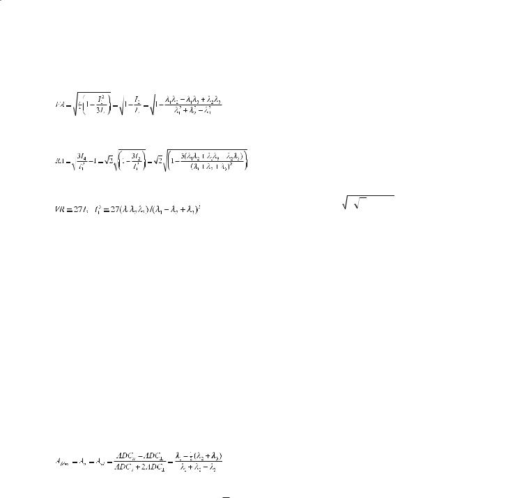
isotropy (RA), and volume ratio (VR), which relate to the invariants via:
range: 0 (isotropic) - 1(anisotropic) |
[6.9a] |
|
|
(anisotropic) |
[6.9b] |
range: 0 (isotropic) –√2 |
|||
range: 1 (isotropic) – 0 (anisotropic) |
[6.9c]. |
Of these, the most commonly used one is the FA, but in principle any of them can be used as they are inherently related (Ulug and van Zijl 1999).Another measure that has been suggested is the so-called lattice anisotropy index (LI) (Pierpaoli and Basser 1996; Pierpaoli et al. 1996), which is an inter-voxel (lattice) measure in which voxel anisotropies are compared to those of neighboring voxels. Obviously, such a comparison depends on spatial resolution and the distance from the voxel and is more complex than the intra-voxel quantities in Eq. 6.9.Another very useful index, which is directly related to the cylindrical symmetry of diffusion is the fiber anisotropy (Ulug and van Zijl 1999), also called the total anisotropy (Aσ) (Conturo et al. 1996) or the standard deviation anisotropy (Asd):
[6.10]
Prolate diffusion range:
1 (anisotropic) – 0 (isotropic): Afiber = RA / √2
Oblate diffusion range:
0 (isotropic) – –0.5 (anisotropic)
An anisotropy index should preferably have the following properties: (a) to have a physical meaning, it should represent inherent diffusion ellipsoid properties; (b) to be measured reproducibly in vivo, it should be orientation independent; (c) to reduce bias and sensitivity to noise, it should not require eigenvalue sorting i.e., the ordering by magnitude;
(d)to avoid introduction of additional noise, it shouldbeobtainablewithouttensordiagonalization;
(e)for improved understanding and convenience, it should be normalized between 0 (isotropic) and 1 (fully anisotropic). These conditions are met by FA,
RA / √2 = Afiber, and 1–VR. One important question relates to the sensitivity of these related indices to
tissue differences in cylindrical anisotropy. Based on their definitions, FA is most sensitive for cylin-
drical anisotropy below 0.5, RA / √2 = Afiber is linear over the full range, and 1–VR is the most sensitive
above 0.85. A better index in the above-0.5 range would therefore be the so-called ultimate volume
anisotropy: UAvol = (33 I3 / I1 − 1)2 (Ulug and van Zijl 1999), which is more sensitive above about
0.6.
Anisotropy measurements are now starting to be used in clinical application. It may not be well realized that these anisotropy numbers can be obtained without tensor diagonalization, but this may lead to simpler techniques in the future.When fiber tracking is the goal of the experiments (see Sect. 6.5), diagonalization of the tensor is still necessary to obtain the eigenvectors.
6.4
DTI Data Acquisition
In a diffusion experiment, magnetic field gradients are used to sensitize the experiment to microscopic tissue water motion. As such, the experiments are extremely sensitive to motion as well as to the performance of the gradients (stability, eddy currents). Most modern imagers have high-quality shielded gradients and can perform excellent single-shot echo planar imaging (EPI). Thus, previous approaches to avoid motion influences, such as the use of navigator echoes and cardiac gating are less common. Recently, the quality of EPI data was further improved by the use of parallel imaging (SENSE,
Pruessmann et al. 1999; SMASH, Sodickson and
Manning 1997) which can remove much of the image distortions due to local field inhomogeneities (Bammer et al. 2002). This has become especially important with the recent more common availability of clinical 3T scanners, because magnetic field inhomogeneity effects scale with the field. Another effect of magnetic field inhomogeneities is the presence of background gradients that interfere with the imaging gradients as well as the diffusion quantification. The imaging gradients themselves can also

Quantitative Diffusion Imaging |
69 |
interfere with the diffusion quantification. This latter problem can simply be solved by placing the dephasing gradients directly next to the encoding and slice-selection gradients, avoiding interference. In the following, we will assume all of these parameters to be acceptable and focus only on the diffusion weighting to be attained for the purpose of trace imaging and the more involved anisotropy imaging and fiber tracking.
For a recent review of DTI data acquisition, see
Basser and Jones (2002)
6.4.1
Trace Imaging
Trace imaging (van Gelderen et al. 1994) is currently the most common application of DTI. In most clinics, this consists of three measurements (x,y,z weighting) and addition of the scans. This will work well, as long as interference with imaging gradients is avoided (see above) and background gradients are limited. Actually, it is possible to perform trace imaging in a single scan in which most interference with background gradients is removed (Mori and van Zijl 1995; Wong et al. 1995; Chung et al. 1998). For correct quantification, it is prerequisite that no interfering imaging gradients are present during diffusion encoding, but this can be easily accomplished as outlined above. The recent availability of imaging gradients as strong as 8 G/cm on whole-body systems may make this sequence more popular, especially in view of the high quality images that can be attained
6.4.2
Anisotropy Imaging
In DTI, acquisition schemes need to be used that acquire all elements of this diffusion tensor in an optimal manner, i.e., as fast as possible and with the highest signal to noise ratio (SNR). Because the tensor is symmetric, DTI requires diffusion weighting along at least six independent axes plus a reference image.The latter should employ some minimal diffusion weighting to remove some unwanted coherence pathways as well as some flowing components (b- value of 50-100 s/mm2). At the high value, weighting in all directions should be sufficient to obtain a wellmeasurable difference. This is not trivial, as signal loss due to weighting may be easily achieved along the fiber direction, but not as easily perpendicular
to it. At present, b-values from 600-1000 s/mm2 are most routinely used. Another factor that has to be optimized is the orientation of the gradients. As one can easily understand, the best combination of gradient orientations, without a priori knowledge of tensor orientation and any bias, is to distribute them uniformly in the 3D space. For example, for six orientations, it becomes an octahedral configuration. Recent important work by Jones et al. (1999b) has shown that optimum acquisition scheme for tensor component determination uses more than six directions, namely about 20-30 (Skare et al. 2000). Importantly, the number of reference scans should also be increased in proportion in order to maintain optimum SNR properties, namely about 1:6 (Skare et al. 2000). At our scanner we presently use 32 directions and 5 references. To avoid motion artifacts, it helps to acquire all directions separately and to align the individual diffusion-weighted images before performing the tensor analysis using multi-variate fitting.
Finally, two important issues have to always be kept in mind. First of all, when working at limited SNR, anisotropy values may increase and thus lead to erroneous interpretation of the data. Secondly, partial volume effects (with CSF or gray matter structures; Alexander et al. 2001; Pfefferbaum et al. 2003) may change the measured anisotropies, which consequently may show a resolution dependent effect. This may cause problems when comparing anisotropies between different research groups or even between normal controls and patients, where some atrophy or different choice of reference slice may be misinterpreted for a lesion. Such problems will obviously worsen for smaller brain structures.
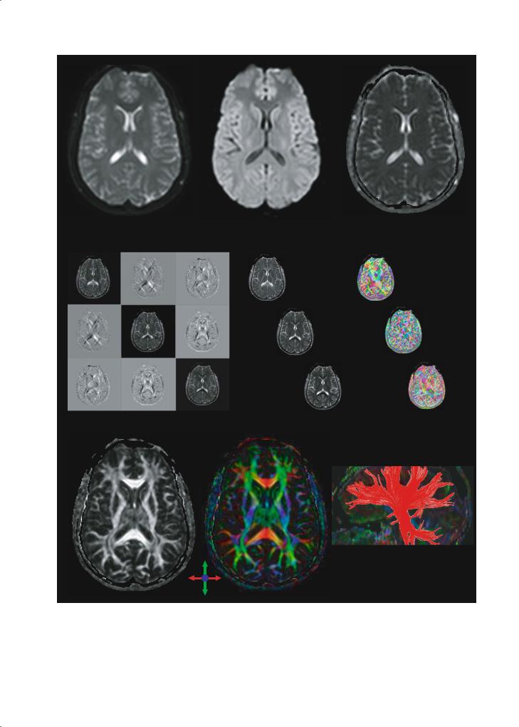
Figure 6.3 demonstrates the types of images that are usually acquired and how the appearance of the image typically changes during data analysis.
The reader is also referred to the works by
Pierpaoli and Basser (1996) and Pierpaoli et al. (1996) for further discussion of anisotropy imaging.
70 |
|
|
|
|
P. C. M. van Zijl et al. |
|
|
|
|
|
|
a |
SD/T2W |
b |
DWI |
c |
ADC av |
d |
= |
|
e |
eigenvalues |
f |
eigenvectors |
||
D (Cartesian coordinates) |
||||||||
ADCxx |
ADCxy |
ADCxz |
|
|
λ1 |
|
vector1 |
|
ADCyx |
ADCyy |
ADCyz |
|
|
λ2 |
|
vector2 |
|
|
|
|
|
|
||||
|
|
|
|
|
|
|
|
|
|
|
|
|
|
|
|
|
|
|
|
|
|
|
D |
|
|
|
ADCzx |
ADCzy |
ADCzz |
|
|
|
λ3 |
vector3 |
|
g Anisotropy map (FA) |
h Color map |
i Fiber map |
Fig. 6.3a–i. Different image types used in DTI. a b0 map (actually b ~ 50 s/mm2); b DWI (b ~ 700 s/mm2); c ADCav map; d tensor images in the cartesian (laboratory) reference frame; e tensor elements remaining after diagonalization, namely the eigenvalues: l1, l2, l3; f eigenvectors; g FA map; h color-coded map showing fibers oriented right–left as red, anterior-posteriorly as green, and perpendicular to the plane as blue; intensity is proportional to FA; i fiber-tracking of the fibers passing through the left middle cerebral peduncle
Quantitative Diffusion Imaging |
71 |
6.5
Axonal Mapping/Fiber Tracking
Another parameter that can be obtained from DTI is the orientation of diffusion ellipsoids (eigenvectors). The most intuitive way to show the orientation is the vectors presentation, in which small lines (vector) indicate the orientations of the longest axis of diffusion ellipsoids. However, unless a small region is magnified, the vector orientation is often difficult to see. To overcome this problem, a color-coded scheme is used (Pajevic and Pierpaoli 1999; Makris et al. 1997). Examples are shown in Fig. 6.4 (left). In the
color map, three orthogonal axes (e.g., right–left, su- perior–inferior, and anterior–posterior) are assigned to three principal colors (red, green, and blue). If a fiber is running at 45º from red and blue axes, it is assigned magenta, which is mixture of red and blue.
Assuming that the orientation of the largest component of the diagonalized diffusion tensor represents the orientation of dominant axonal tracts, DTI can provide a 3D vector field, in which each vector presents the fiber orientation (Fig. 6.4). Currently, there are several different approaches to reconstruct white matter tracts, which can be roughly divided into two types. Techniques classified in the first category are
sfo |
|
slf |
|
|
|
ifo
|
|
ilf |
|
unc |
|||
|
|
||
|
|
|
l
scrscr
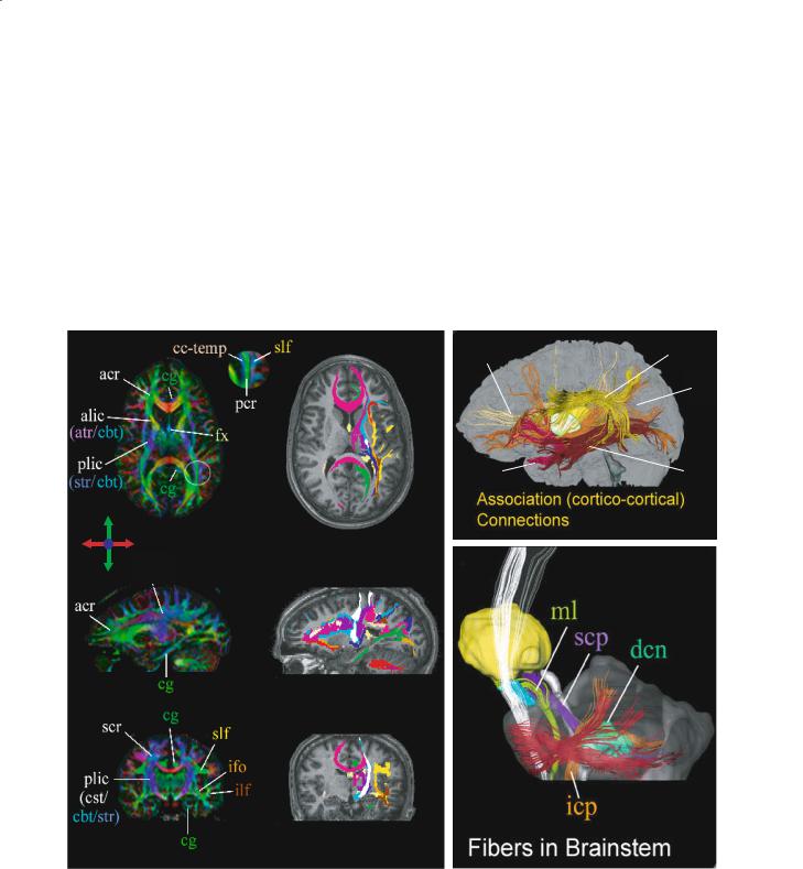
Fig. 6.4. Examples of brain fiber color maps (left column) and 3D-based fiber tracts projected in a plane (middle column) or shown in 3D space (right column). In the color maps, blue, red, and green indicate inferior (i)–superior (s), left–right, and anterior (a)–posterior, respectively. The 3D fiber tracts in the middle column are superimposed on MPRAGE images, showing that axonal mapping can be used to parcelate the white matter. acr, Anterior corona radiata; alic, anterior limb internal capsule; atr, anterior thalamic radiation; cbt, corticobulbar tract; cg, cingulum; cp, cerebellar peduncle; cst, corticospinal tract; dcn, deep cerebellar nuclei; fx, fornix; icp, inferior cerebellar peduncle; ifo, inferior fronto-occipital fasciculus; ilf, inferior longitudinal fasciculus; ml, medial lemniscus; pcr, posterior corona radiate; plic, posterior limb internal capsule; scp, superior cerebellar peduncle; scr, superior corona radiata; sfo, superior fronto-occipital fasciculus; slf, superior longitudinal fasciculus; str, superior thalamic radiation; unc, uncinate fasciculus. [Data reproduced with permission from Wakana et al. (2004)]

72 |
P. C. M. van Zijl et al. |
based on line propagation algorithms that use local tensor information for each step of the propagation. The main differences among techniques in this class stem from the way information from neighboring pixels is incorporated to define smooth trajectories or to minimize noise contributions. The second type of approach is based on global energy minimization to find the energetically most favorable path between two predetermined pixels. These methods have been recently reviewed (Mori and van Zijl 2002), but many more innovations and improvements are expected in the coming years. When designing or using such technologies, it is important to understand the basis of the anisotropy contrast in DTI and the limitations imposed by using a macroscopic technique to visualize microscopic restrictions.For instance,when using such vector fields to track axonal pathways, one must always be aware of the influence of noise, partial volume effects and the effect of termination criteria (Mori and van Zijl 2002; Lori et al. 1999, 2002;
Mangin et al. 2002; Lazar and Alexander 2001). The following main points should be kept in mind. First, conventional DTI data acquisition and processing methods are challenged by a voxel containing more than one population of axonal tracts with different orientations. Second, DTI cannot provide information on cellular-level axonal connectivity. Multiple axons from individual cells may merge into or branch out from one voxel.Within a voxel, cellularlevel axonal information of multiple compartments is averaged. The third important limitation is that afferent and efferent pathways of axonal tracts cannot be judged from the direction of water diffusion in a voxel. The question that often arises is therefore what tractography will be able to provide. Based on the relative size of the voxel and the human brain and recent experimental results (Wakana et al. 2004), it should be safe to say that it can rev matter tracts (e.g., see the atlas data in Fig. 6.3). The possibility to study crossing fibers has also been suggested (Frank 2001; Tuch et al. 2001; Wiegell et al. 2000), but more research is needed in this area.
6.6
Applications of Quantitative DWI/DTI to the Brain
Most applications were recently reviewed in an article by Dong et al. (2004), and in special issues of NMR in Biomedicine (Vol. 15, issues 7,8, 2002) and the European Journal of Radiology (Vol. 45, issue 3,
2003). As mentioned in the introduction, the structural organization of the brain comprises multiple microscopic components, including microtubules, cell membranes, axons, myelin, and macromolecules arranged into macroscopically identifiable structures such as the fiber bundles. This architecture restricts the Brownian motion of water, superimposing varying degrees of anisotropy depending on the location in the brain. Diffusion, probing this water motion, therefore yields an in vivo measurement of a physical property rather than an MRI property such as T1, T2 and magnetization transfer (Horsfield and Jones 2002). An alteration of such a physical property in case of disease can represent a distinct and advantageous window for clinical analysis. Thus, because microscopic information is provided by this technique, a higher sensitivity for lesion detection is expected, either in diseases bearing focal lesions or diffuse abnormalities. Such a higher sensitivity compared to conventional MRI would allow early intervention, which is considered to be crucial in diseases such as stroke. Refinement of diagnosis with more precise anatomical information, for instance, involvement of surrounding anatomical structures in tumors and more precise localization of lesions will lead to better correlations with clinical scales. This may offer substantial benefits to patients including potentially better treatment choices and improved follow-up information.
6.6.1
Normal Control Values of Di usion Parameters During Early Development and Aging
Although studies that evaluate focal lesions usually use the correspondent contralateral areas for comparison, studies that include more diffuse lesions commonly need their own group of normal controls. Tables 6.2 and 6.3 summarize normative anisotropy
(FA and Afiber = RA / √2 ) and average apparent diffusion coefficient (ADCav) values reported in the litera-
ture for several structures in white matter (WM) and gray matter (GM), respectively. The average diffusion constant was first used in the stroke literature (Mori and van Zijl 1995; Decanniere et al. 1995) and is defined by:
ADCav |
= Tr( |
D |
)/3 |
[6.11] |
|
|
|
|
Even though (ADCav, FA, and Afiber are orientationindependent quantities, care has to be taken in their
interpretation. The reason is the influence of partial