Книги по МРТ КТ на английском языке / MR Imaging in White Matter Diseases of the Brain and Spinal Cord - K Sartor Massimo Filippi Nicola De Stefano Vincent Dou

water (Phelps 1991), nuclear medicine SPECT studies of 133Xe (Jaggi et al. 1993), and X-ray CT studies of stable xenon (Wintermark et al. 2001) all provide maps of rCBF. The American Heart Association has recently compiled guidelines and recommendations for perfusion imaging in ischemic brain disease (Latchaw et al. 2003).

In the last 15 years, advances in MRI have led to more and more routine and common measures to assess of CBF by MRI. Within MRI, DSC and ASL account for the vast majority of studies in the literature. DSC imaging uses a bolus injection of contrast agent and measures rCBF by following the time course of signal change in the brain caused by the passing of the bolus through an imaging voxel (Villringer et al. 1988; Rosen et al. 1989; Belliveau et al. 1990, 1991). DSC MRI is used in most clinical MRI studies because of the high signal-to-noise ratio of the method and the ease of obtaining a relative (as opposed to absolute) measure of CBF. ASL methods magnetically label the blood flowing into the brain and create a new steady-state level of magnetization (Detre et al. 1992; Williams et al. 1992; Kim 1995). ASL has the advantage that it uses no contrast agent but labels or tags water molecules by RF saturation. Because ASL does not use contrast agents, it is entirely non-invasive and may be repeated often. ASL is used in animal studies and in volunteer, or task activation functional imaging studies. There is a price to pay, however, as the signal-to-noise ratio (SNR) of the ASL perfusion image is approximately ten times less than the SNR of the DSC perfusion image. Other MRI methods are also being developed to measure rCBF. One promising technique is laser polarized xenon MRI (Swanson et al. 1997). Xenon has long been used to measure CBF with SPECT or X-ray CT. Laser polarized xenon MRI has recently been used to measure CBF by Duhamel et al. (2002).

7.3

Dynamic Susceptibility Contrast

DSC MRI measures the passage of a bolus of non-dif- fusible contrast through the brain.A bolus of contrast is injected into a vein and travels through the vasculature into the brain where the change in MRI signal is recorded. The signal decreases as the bolus passes through the imaging slice. The decreased signal change is mathematically converted to a change in the concentration of contrast agent. The time course of the rate of change of contrast agent is integrated

to yield the relative cerebral blood volume (relCBV). The arterial signal is also recorded and used to compute the mean transit time (MTT) and rCBF (regional cerebral blood flow).

7.3.1

What Causes the Signal to Change?

Signal intensity decreases because the paramagnetic contrast disrupts the magnetic fields in a small region surrounding the capillaries as it passes through the tissue. Disruption of the magnetic field decreases T2* (or increases R2*= 1/T2*) of water protons in tissue near the contrast agent. Since the echo of the spins is recorded at a time TE following the pulse, the change in T2* will result in a decrease in the signal intensity of the water proton spins.

The intensity of the water proton signal at time TE will be given by:

where R2 is the transverse relaxation rate (1/T2) of tissue. R2* is the effective transverse relaxation rate (1/T2*) in the presence of contrast agent.

If contrast agent is added to the tissue, an additional relaxation occurs due to the susceptibility induced dispersion created by addition of paramagnetic ions. The new relaxation rate can be defined as:

where r2* is the relaxivity (relaxation rate per unit concentration of gadolinium) and CGd(t) is the time dependent concentration of the gadolinium contrast agent. Rate constants (rather that the time constants such as T2 are used because the rates are additive and simplify the math. The signal intensity at time TE is now defined as:

7.3.2

How Does the Signal Change Correspond to Tracer Concentration?

The goal of this procedure is to calculate the concentrate of the concentration of the tracer. This can be done by taking the logarithm of the ratio of the signal with and without contrast agent.

MR Methods to Measure Cerebral Perfusion

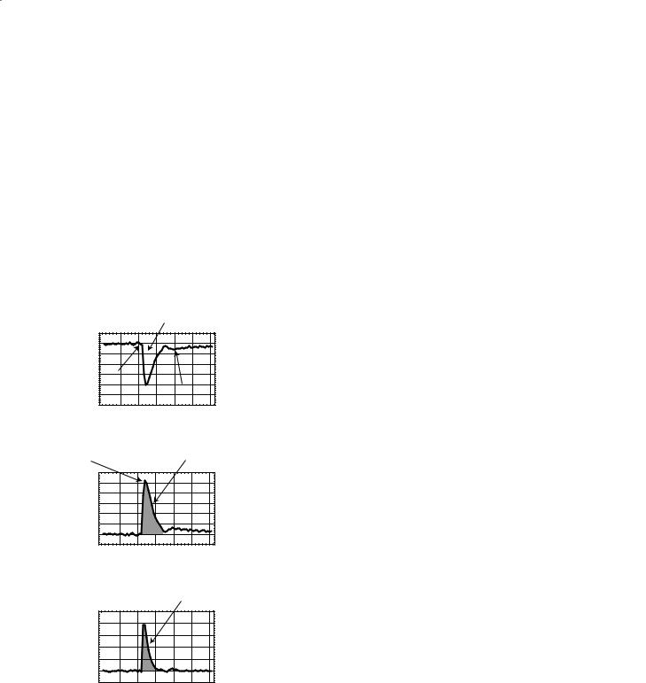
Figure 7.1a shows a representative curve of the signal intensity in a voxel as the contrast agent passes through the volume. These data are processed with Eq. (7.5) to generate the time–concentration curve shown in Fig. 7.1b. The arterial input function (AIF) (Fig. 7.1c) is measured from voxels near a major artery such as the MCA.

Signal decreases as Gd bolus passes through

imaging voxel

Fig. 7.1a–c. Generation of the concentration–time curve. The passage of contrast agent through the voxel causes the signal to decrease due to a decrease in T2* (an increase in R2*) resulting in a decrease in the MR signal (a). The signal–time curve is turned into a concentration–time curve by using equations 7.4 and 7.5. The arterial input function (c) is created in a similar manner, using these same equations to transform the signal–time curve measured near a major artery into a concentration–time curve.

85

Because the bolus passes through the tissue in a very short time, echo planer imaging (EPI) methods are needed to image the profile seen in Fig. 7.1a (Kwong et al. 1995).

This procedure assumes that the contrast agent does not leak out of the vessels into the tissue and that the contrast agent causes insignificant T1 enhancement.

7.3.3

How Is the Time–Concentration Tracer Curve Turned into a Measure of Perfusion?

After recording the images and creating the time– concentration curves for each voxel or region of interest, the data needs to be further analyzed to create maps of perfusion (rCBF), MTT, and CBV. At this stage the investigator needs to decide whether he or she desires a relative or a quantitative map of perfusion. There are basically three paths: (1) numerical integration (or summing up) of the data to create relative maps of CBV; (2) fitting the data to a gammavariant function; or (3) deconvolution of the data using the AIF (Perkio et al. 2002). Of these three methods we will consider numerical integration and deconvolution.

7.3.3.1

Numerical Integration

The easiest method to create a measure of perfusion is to measure the area of the time–concentration curve (Fig. 7.1b).

This will provide an index that is proportional to the relative cerebral blood volume (relCBV) of a given pixel. Because of the ease of performing the numerical integration, this method is perhaps the most used in clinical application of MR perfusion imaging. It should be noted that this does not provide an absolute, quantitative measure of cerebral blood volume, but yields an image that may be useful for comparing normal to ischemic or diseased tissue.

7.3.3.2 Deconvolution

Indicator-dilution theory of perfusion imaging for non-diffusible tracers states that the time–concentra- tion profile is equal to the cerebral blood flow times

the convolution of the AIF and the tissue residue function (Meier and Zierler 1954; Zierler 1965).

If the reader understands this equation and all of its implications, then read no further. If, however, one is trying to gain an understanding of how this convolution integral can be used to measure perfusion, then this section should be very helpful.

This statement leads to three obvious questions: What is the arterial input function? What is a convolution integral? What is a residue function?

The arterial input function was introduced previously and is simply the concentration of contrast agent in the arteries as a function of time. In a perfect world, one could shape the arterial input function so that it would be a delta function, or instantaneous spike of contrast agent. This would greatly simplify the mathematics and make quantitative perfusion imaging trivial. Because of the realities of injection and diffusion of contrast agent within the blood, this ideal function can never be achieved in practice. In general the AIF is a broad, Gaussian-like function determined by the rate at which contrast agent is injected and by the spread of the contrast agent that occurs as the blood flows from the injection site to the brain.

The second term, the residue function, is the manner in which contrast agent is retained by the tissue. Because there are many pathways that molecules of Gd chelates can follow through the capillary bed to leave the tissue, the residue function is a statistical probability of how it is retained in the tissue. The residue function is determined by deconvolving the time–concen- tration function with the arterial input function.

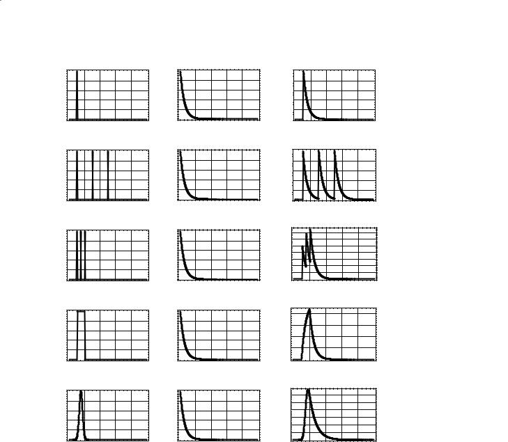
Figure 7.2 demonstrates convolution. The left column contains different arterial input functions ranging from a delta function in Fig. 7.2a to a Gaussian function in Fig. 7.2e. The center column contains an exponentially decaying residue function and is the same for each row. The right column shows what the detected tissue MRI signal would be measured for these combinations of AIF and residue functions. The delta function AIF in Fig. 7.2a is shifted by 10 s. Convolution of this function with the exponentially decaying residue function simply shifts the residue function by 10 s. In Fig. 7.2b, the AIF contains three well separated delta functions. Convolution with the residue function creates three well-separated exponentially decaying functions. As the delta functions become closer in time (Fig. 7.2c), the measured re-

sponse does not decay to zero before another bolus of signal arrives. Therefore, the signal builds up with each additional arrival of bolus. In Fig. 7.2d, the AIF is a square wave (a series of back-to-back delta functions). The measured tissue response builds up while the AIF has a value of 1, and decays when the AIF = 0. Note change in scale in the value of the measured response in Fig. 7.2d. Finally, a more realistic Gaussian function is used in Fig. 7.2e for the AIF.

The demonstration of convolution in Fig. 7.2 does not show one how to deconvolve. Deconvolution is a much more complicated process and beyond the scope of this chapter. In summary, deconvolution uses an iterative process to create an estimate of the residue function if one is given the AIF and the time–concen- tration curve in the tissue of interest (Ostergaard et al. 1999). From Eq. (7.7), one can see that once the AIF and the residue function are known, then one can calculate a quantitative estimate of CBF.

u=0

Since we have measured the time–concentration curve and the AIF, a quantitative estimate of CBF can be made.

∫ AIF(t)dt

Where is a scaling factor depending on the hematocrit and vessel geometry. Moreover, from the central volume theorem (Meier and Zierler 1954), one can calculate the mean transit time (MTT).

Deconvolution of the time–concentration curve with the AIF provides quantitative estimates of CBF, CBV, and MTT.

7.4

Arterial Spin Labeling

Arterial spin labeling (ASL) magnetically labels the water proton spins in blood that is flowing into the brain (Detre et al. 1992). Either continuous wave (CW) or pulsed (Kim 1995) RF energy is used to selec-

MR Methods to Measure Cerebral Perfusion

87

measured response

1

0.8

0.6

0.4

0.2

0

1

0.8

0.6

0.4

0.2

0

Intensity

Intensity

Intensity

tively invert magnetization in the arteries. Numerous methods have been developed over the last 10 years and are well reviewed in Calamante et al. (1999) and Barbier et al. (2001). This work focuses on the fundamental equations of sources and sinks of magnetization in the brain and illustrates the complicated coupled differential equations describing ASL imaging with simple pictures of coupled reservoirs.

7.4.1

What Causes the Signal to Change?

In order to be effective, ASL methods label the water proton magnetization in the blood stream to create a signal difference in the region of interest. The labeling is done with either CW RF excitation or with a pulsed RF excitation.

88

7.4.1.1

Spin-Lattice Relaxation

To gain an understanding of how ASL methods work, one must first examine the basic equations of magnetization. The Bloch equations state that the rate of change of magnetization is proportional to the difference between the equilibrium magnetization and the current level of magnetization. In a static sample, with no inflowing water molecules, magnetization is restored to equilibrium values by random motions of the nuclear spins. The time constant for this process is, of course, T1. Mathematically, this is written as a first order differential equation.

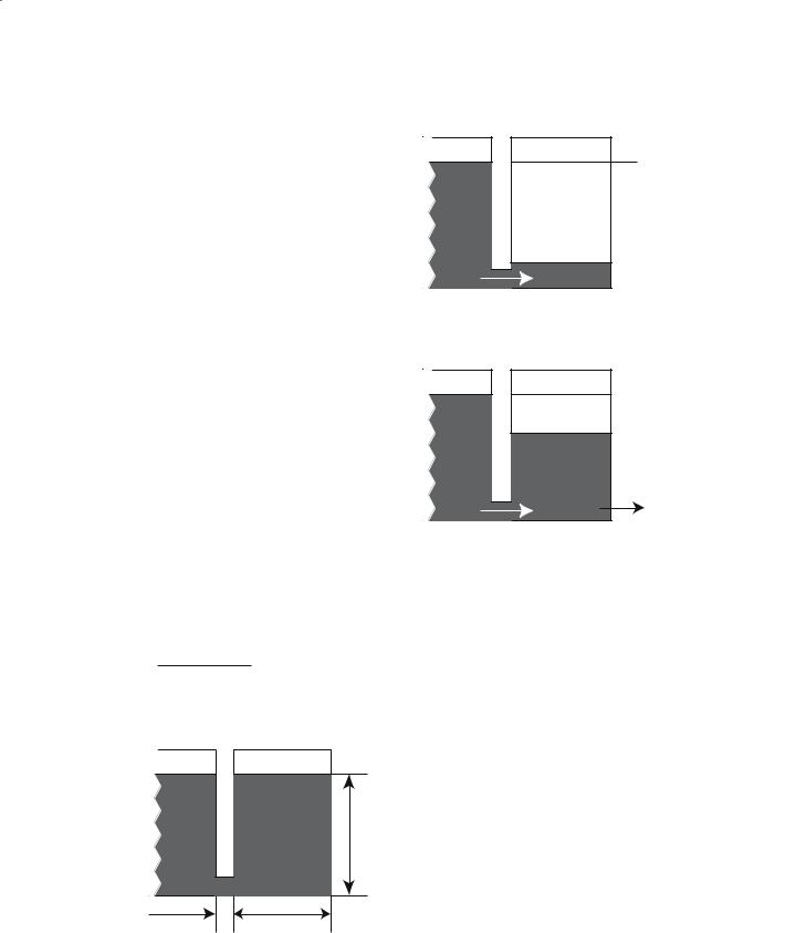
where Mz(t) is the time-dependent value of longitudinal magnetization, M0 is the equilibrium value, and T1 is the spin-lattice relaxation time constant. Figure 7.3 shows a schematic of Eq. (7.11), where the reservoir of tissue magnetization is coupled to an infinite “lattice” by the rate constant R1.

Figure 7.4a demonstrates what happens when the tissue magnetization is saturated by an RF pulse. Magnetization will flow from the lattice, with rate constant R1, until the tissue reservoir is filled to M0. Figure 7.4b shows that if Mz(t) is sampled at times TR with a pulse of flip angle δ, the steady-state, longitudinal magnetization will be

width of lattice is infinate width = volume of sample

signal size = width x height = total magnetization

Fig. 7.3. Coupled reservoirs model of nuclear magnetization in a static sample

S. D. Swanson

aT1 recovery of magnetization

Mo

Mz is depleted by RF pulsing and is replenished by spinlattice relaxation.

a

bSteady-state magnetization

Fig. 7.4a,b. Coupled reservoir model of magnetization following inversion (a) and during RF pulsing (b)

7.4.1.2

Coupled Reservoirs of Magnetization

In vivo, there are other sources and sinks of water proton magnetization. One source would be the arterial blood flowing into a region of tissue and one sink would be the flow of venous blood exiting the tissue. The differential equation could then be written as,

Because water is a freely diffusible tracer, the value of the magnetization in the venous blood can is given by the magnetization in the brain divided by the partition coefficient.

where F is the blood flow in ml/100g/min, λ is the blood/brain partition coefficient for water.

An additional magnetic coupling in brain tissue is the magnetization transfer that occurs between the mobile water protons and the immobile lipid bilayer protons of white and gray matter. MT is generated by applying RF energy off-resonance from the narrow water proton line but within the linewidth of the broad lipid proton resonance.The RF energy partially saturates the magnetization of the solid-like protons. This saturation is transferred to the water protons by magnetic cross-relaxation and exchange. MT occurs in ASL because the CW RF needed to invert magnetization in the carotid arteries causes significant MT in the brain. Therefore a control RF pulse is needed that generates MT but does not label arterial blood (Mclaughlin et al.1997).Pulsed methods minimize, but do not eliminate, MT effects in ASL. MT can be included by adding a term for cross-relaxation between the mobile and immobile protons

where R1 is the cross relaxation rate.

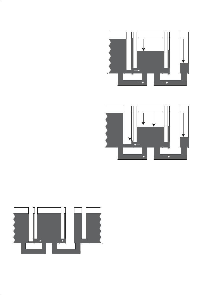
Figure 7.5 provides a picture of all of the magnetic couplings and magnetization flow patterns that are described mathematically in Eq. (7.15).

7.4.2

Measurement of Flow with ASL

Figure 7.6 demonstrates the conditions for CW ASL. In Fig. 7.6a, a control RF pulse is applied along with a magnetic field gradient. The pulse is off-resonance for spins in the brain and creates significant MT effect, resulting in a decrease in brain tissue signal. In

Fig. 7.5. A complete model of the coupled reservoirs of magnetization in the brain

Fig. 7.6a,b. Behavior of magnetization during the control CW RF irradiation (a) and ASL of the carotid arteries (b)

Fig. 7.6b, the same RF energy is applied to the brain causing the same MT effect. This pulse, however, is on-resonance for spins in the carotid arteries and inverts the magnetization of the spins flowing into the brain. Because the level of magnetization in the arteries is less than the level of magnetization in the brain,the net flow of magnetization is out of the brain causing an additional decrease in the brain signal. The difference between the saturation in Fig. 7.6a and Fig. 7.6b is given by Williams et al. (1992):

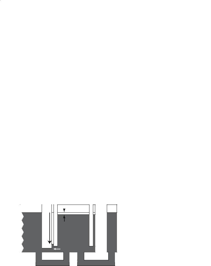
To obviate the problems of MT, one needs to use a separate RF surface coil on the carotid arteries (Silva et al. 1995). This is technically challenging but allows one to label the water protons in the carotid arteries without causing MT in the brain. A schematic example of this technique is shown in Fig. 7.7.

7.5

Laser Polarized Xenon

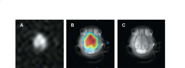
Alternative means to measure CBF using MRI are also being explored. One promising technique that has been used in small animal models is laser polarized or hyperpolarized 129Xe (Fig. 7.8) (Swanson et al. 1997; Duhamel et al. 2002). Xenon is a freely diffusible tracer and has been used by both CT (by attenuation of X-rays) and SPECT (as radioactive 133Xe) to measure rCBF. Laser polarization increases the nuclear polarization (the percent of xenon in the spin up state) from normal levels of about 0.0001% to approximately 50% in ideal cases. With increased MR signal and near ideal tracer kinetics, it should be possible to use MRI of laser polarized xenon to measure perfusion.

For a freely diffusible tracer, such as xenon, the time–concentration profile of xenon in the tissue will be given by the same convolution integral [Eq. (7.7)] examined earlier.

Though it is informative to evaluate the longitudinal magnetization, as done in Eq. (7.17), the imaging experiment will measure the transverse magnetization and it is necessary to determine the transverse magnetization.This is especially critical for polarized gas MRI, as the MR signal will be destroyed with each additional pulse. This fact is both a disadvantage and an advantage when attempting to measure flow with polarized gas MRI. It is a disadvantage in that once the magnetization is destroyed, it is gone and will not be replaced by T1 processes. It is an advantage because the ability to destroy the signal of the tracer that we are using to measure flow means that there will be no problem with recirculation of tracer. Once the signal is used, it is gone.

With a constant arterial input function, one can show that the transverse xenon magnetization will be:

With appropriate RF pulsing, the detected xenon signal in Eq. (7.18) linearly proportional to flow. Though rCBF measurements with laser polarized xenon are currently challenging, further advances in polarization technology and delivery may show that this historically important atom may yet have a role to play in MR methods to measure cerebral perfusion.

Fig. 7.7. Behavior of magnetization during CW RF irradiation using a dedicated surface coil in the neck. MT effects are eliminated.

References

Barbier E, Lamalle L, Decorps M (2001) Methodology of brain perfusion imaging. J Magn Reson Imaging 13:496-520 Belliveau J, Rosen B, Kantor H, Rzedzian R, Kennedy D, Mck-

instry R, Vevea J, Cohen M, Pykett I, Brady T (1990) Functional cerebral imaging by susceptibility-contrast NMR. Magn Reson Med 14:538-546

Belliveau J, Kennedy DJ, Mckinstry R, Buchbinder B, Weisskoff R, Cohen M, Vevea J, Brady T, Rosen B (1991) Functional mapping of the human visual cortex by magnetic resonance imaging. Science 254:716-719

Calamante F, Thomas D, Pell G, Wiersma J, Turner R (1999) Measuring cerebral blood flow using magnetic resonance imaging techniques. J Cereb Blood Flow Metab 19:701-735 Detre J, Wang J (2002) Technical aspects and utility of fMRI

using bold and ASL. Clin Neurophysiol 113:621-634

Detre J, Leigh J, Williams D, Koretsky A (1992) Perfusion imaging. Magn Reson Med 23:37-45

Duhamel G, Choquet P, Grillon E, Leviel J, Decorps M, Ziegler A, Constantinesco A (2002) Global and regional cerebral blood flow measurements using NMR of injected hyperpolarized xenon-129. Acad Radiol 9 [Suppl 2]:S498-500

Hunsche S, Sauner D, Schreiber W, Oelkers P, Stoeter P (2002) Fair and dynamic susceptibility contrast-enhanced perfusion imaging in healthy subjects and stroke patients. J Magn Reson Imaging 16:137-146

Jaggi JL, Obrist WD, Noordergraaf A (1993) Signal analysis of noninvasive xenon-133 cerebral blood flow measurements. Ann Biomed Eng 21:85-95

Kety SS, Schmidt CF (1945) The determination of cerebral blood flow in man by the use of nitrous oxide in low concentrations. Am J Physiol 143:53-66

Kim S (1995) Quantification of relative cerebral blood flow change by flow-sensitive alternating inversion recovery (FAIR) technique: application to functional mapping. Magn Reson Med 34:293-301

Kwong K, Chesler D, Weisskoff R, Donahue K, Davis T, Ostergaard L, Campbell T, Rosen B (1995) MR perfusion studies with T1-weighted echo planar imaging. Magn Reson Med 34:878-887

Latchaw R, Yonas H, Hunter G, Yuh W, Ueda T, Sorensen A, Sunshine J, Biller J, Wechsler L, Higashida R, Hademenos G (2003) Guidelines and recommendations for perfusion imaging in cerebral ischemia: a scientific statement for healthcare professionals by the writing group on perfusion imaging, from the council on cardiovascular radiology of the american heart association. Stroke 34:10841104

Mclaughlin A, Ye F, Pekar J, Santha A, Frank J (1997) Effect of magnetization transfer on the measurement of cerebral blood flow using steady-state arterial spin tagging approaches: a theoretical investigation. Magn Reson Med 37:501-510

Meier P, Zierler K (1954) On the theory of the indicator-dilu- tion method for measurement of blood flow and volume. J Appl Physiol 6:731-744

Ostergaard L, Weisskoff R, Chesler D, Gyldensted C, Rosen B (1996) High resolution measurement of cerebral blood flow using intravascular tracer bolus passages, part I: mathematical approach and statistical analysis. Magn Reson Med 36:715-725

Ostergaard L, Sorensen A, Kwong K, Weisskoff R, Gyldensted C, Rosen B (1996) High resolution measurement of cerebral blood flow using intravascular tracer bolus passages, part II: experimental comparison and preliminary results. Magn Reson Med 36:726-736

Ostergaard L, Chesler D, Weisskoff R, Sorensen A, Rosen B (1999) Modeling cerebral blood flow and flow heterogeneity from magnetic resonance residue data. J Cereb Blood Flow Metab 19:690-699

Perkio J,Aronen H, Kangasmaki A, Liu Y, Karonen J, Savolainen S, Ostergaard L (2002) Evaluation of four postprocessing methods for determination of cerebral blood volume and mean transit time by dynamic susceptibility contrast imaging. Magn Reson Med 47:973-981

Phelps ME (1991) PET - a biological imaging technique. Neurochem Res 16:929-940

Rosen B, Belliveau J, Chien D (1989) Perfusion imaging by nuclear magnetic resonance. Magn Reson Q 5:263-281 Rosen B, Belliveau J,Vevea J, Brady T (1990) Perfusion imaging with NMR contrast agents. Magn Reson Med 14:249-265

92

Roy C, Sherrington CS (1890) On the Regulation of the blood supply of the brain. J Physiol 11:85-108

Silva A, Zhang W, Williams D, Koretsky A (1995) Multi-slice MRI of rat brain perfusion during amphetamine stimulation using arterial spin labeling. Magn Reson Med 33:209214

Sorensen A, Copen W, Ostergaard L, Buonanno F, Gonzalez R, Rordorf G, Rosen B, Schwamm L, Weisskoff R, Koroshetz W (1999) Hyperacute stroke: simultaneous measurement of relative cerebral blood volume, relative cerebral blood flow, and mean tissue transit time. Radiology 210:519-527

Swanson S, Rosen M, Agranoff B, Coulter K, Welsh R, Chupp T (1997) Brain MRI with laser-polarized 129Xe. Magn Reson Med 38:695-698

Thomas D, Lythgoe M, Pell G, Calamante F, Ordidge R (2000) The measurement of diffusion and perfusion in biological systems using magnetic resonance imaging. Phys Med Biol 45:R97-R138

Villringer A, Rosen B, Belliveau J, Ackerman J, Lauffer R,

S. D. Swanson

Buxton R, Chao Y, Wedeen V, Brady T (1988) Dynamic imaging with lanthanide chelates in normal brain: contrast due to magnetic susceptibility effects. Magn Reson Med 6:164-174

Weber M, Gunther M, Lichy M, Delorme S, Bongers A, Thilmann C, Essig M, Zuna I, Schad L, Debus J, Schlemmer H (2003) Comparison of arterial spin-labeling techniques and dynamic susceptibility-weighted contrast-enhanced MRI in perfusion imaging of normal brain tissue. Invest Radiol 38:712-718

Williams D, Detre J, Leigh J, Koretsky A (1992) Magnetic resonance imaging of perfusion using spin inversion of arterial water. Proc Natl Acad Sci USA 89:212-216

Wintermark M, Maeder P, Thiran JP et al (2001) Quantitative assessment of regional cerebral blood flows by perfusion CT studies at low injection rates: a critical review of the underlying theoretical models. Eur Radiol 11:1220-1230

Zierler KL (1965) Equations for measuring blood flow by external monitoring of radioisotopes. Circ Res 16:309-321

8Functional MRI

Peter Jezzard and Ahmed Toosy

CONTENTS

8.1Introduction 93

8.2.1Metabolic and Haemodynamic Correlates of Brain Activity 93

8.2.2BOLD Mechanisms 95

8.2.3Other MR-Accessible Markers of Functional Activity 97

8.3Acquisition Practicalities 99

8.3.3The Scanner as a Psychophysical

Testing Environment 103

8.4Experimental Design 103

8.4.1 Block Design Paradigms 103

8.4.2Event-Related Designs 104

8.5.1Pre-Statistics Procedures 105

8.5.2Time-Course Modelling 105

8.5.3Statistical Inference 106

8.7Clinical Applications in White Matter Disorders 107

8.7.1Cortical Plasticity 107

8.8Conclusion 109 References 110

haemodynamic variable to be accessed by functional MRI (fMRI) is the level of blood oxygenation (in fact the MRI signal is sensitive to the level of blood deoxygenation), although MRI is able to access other markers of brain activity.

The majority of fMRI studies to date have addressed questions in basic neuroscience, and have studied the operation of the healthy brain in normal volunteers. A small, but increasing, number of studies have addressed questions in clinical neuroscience, and some of this work has gone on to find application in the clinic (Thulborn and Gisbert 2001). Of this work, little has been directed towards white matter diseases. This is presumably because fMRI methods are generally only sensitive to metabolic, and hence signalling, activity that occurs within the grey matter, and is unable to detect directly the transmission of signal within white matter fibres. Nevertheless, an important new insight into white matter disorders can be achieved by studying the effects on grey matter networks arising from disorders of the white matter.

8.1 Introduction

Developments in magnetic resonance imaging (MRI) over the past decade have demonstrated that MRI, a non-invasive and widespread technology, can also report on human brain function via the correlate of the brain’s associated local haemodynamic response (Belliveau et al. 1991; Ogawa et al. 1992; Kwong et al. 1992; Bandettini et al. 1992). The most common

P. Jezzard, PhD

FMRIB Centre, Department of Clinical Neurology, John

Radcliffe Hospital, Oxford, OX3 9DU, UK

A. Toosy, MD

Department of Headache, Brain Injury and Rehabilitation,

Institute of Neurology, Queen Square, London, WC1N 3BG,

UK

8.2

Physiological and Biophysical Origins of fMRI

8.2.1

Metabolic and Haemodynamic Correlates of Brain Activity

Neurons communicate via small electrical impulses, receiving signals from other neurons via their dendrites, and sending impulses to other neurons via their axon. The signals received via the dendrites may either be excitatory (in which case there is an increased tendency for the neuron to relay the electrical signal further via its axon), or may be inhibitory (in which case there is a decreased tendency for the neuron to relay the electrical signal). Figure 8.1 shows a schematic diagram of a neuron, showing its