Книги по МРТ КТ на английском языке / MR Imaging in White Matter Diseases of the Brain and Spinal Cord - K Sartor Massimo Filippi Nicola De Stefano Vincent Dou

Fig. 8.1. Schematic diagram of a neuron, showing its dendrites, which receive electrical signals from other neurons, and its axon, which relays signals on to other neurons. Connection between neurons occurs across synapses.

principal elements. Surrounding the neurons are glia, which are cells involved in energy metabolism, storage, and maintenance of ionic balance.

The metabolic turnover of glia, activation of neurons, and establishment of the ion potentials in the cells of the brain all require a supply of energy. Current evidence suggests that most of the metabolic demands of brain signalling involve presynaptic activity (input and intracortical processing) rather than soma spiking activity (Logothetis et al. 2001). This energy is supplied in the form of adenosine triphosphate (ATP) generated in the mitochondria within cells. Under normal conditions ATP is formed via glucose consumption in the presence of oxygen (via aerobic glycolysis), and this glucose and oxygen is supplied by blood perfusing the tissue. Previous experiments involving a number of modalities have shown that local glucose consumption rises sharply when neuronal activation takes place. This is accompanied by an increase in local blood flow, and in local blood volume. From the perspective of fMRI, however, it is the balance of oxygen delivery and utilization that results in the observed signal changes. This is because blood oxygen is predominantly transported within red blood cells, bound to the large iron-containing molecule, haemoglobin. As is discussed below, it is the changing magnetic properties of haemoglobin as it gives up its oxygen that provides the most utilized contrast mechanism in functional MRI. Other related physiological parameters that can be accessed by MRI include cerebral blood flow, cerebral blood volume and, in animal models, glucose turnover via carbon-13 spectroscopy.

When considering the oxygen requirements of the brain it is informative to consider a formulation of the Fick principle that relates consumption of a nutrient by a tissue to the arteriovenous difference in the concentration of the nutrient in the blood. In this

case oxygen is assumed to be consumed metabolically, and the Fick principle can be expressed as:

where CMRO2 is the metabolic rate of oxygen consumption, CBF is the cerebral blood flow, [HbTOT] is the total (oxygenated or deoxygenated) concentration of haemoglobin, and the factor 4 accounts for the fact that four oxygen molecules can bind to each haemoglobin molecule. Ya and Yv are the oxygen saturation values (range 0 to 1) for arterial and venous blood (oxygen saturation is the fraction of haemoglobin molecules that are in the oxygenated state), and hence (Ya–Yv) is a measure of the oxygen extraction fraction (OEF).

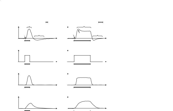
The hypothesized relationship between local CMRO2 and CBF during neuronal stimulation is shown in Fig. 8.2. The increase in local CMRO2 is thought to be rather modest (5–20%) and is coincident with the period of neuronal activity. The increased metabolic demand causes the CBF to increase quite markedly (albeit sluggishly), yielding a peak CBF demand some 5–10 seconds after the onset of stimulation. The increase in local CBF is much more significant (typically 30–100%), a necessary overcompensation that is likely to be due to the limited oxygen diffusion capacity from the blood to the mitochondria (Buxton and Frank 1997). Through Eq. 1 it can be seen that since CBF rises more than CMRO2 during stimulation there is predicted to be a decrease in OEF (i.e. Yv is increased). This is the effect that is used in blood oxygenation level dependent (BOLD) fMRI experiments.

Also shown in Fig. 8.2 is a representation of the associated change in local cerebral blood volume (CBV), along with the observed BOLD fMRI response, for both a short duration and a long duration stimulus. It can be seen that the CBV haemodynamic response is even more sluggish than the CBF haemodynamic response, and indeed contributes to the non-linear overshoot and post-stimulus undershoot that is frequently observed in practical fMRI data sets.The initial dip that is occasionally observed immediately following stimulus onset (Ernst and Hennig 1994; Menon et al. 1995) is postulated to be evidence of the brief temporal uncoupling of oxygen consumption (associated with the CMRO2 increase) and oxygen delivery (associated with the more sluggish CBF increase) leading to a transient blood deoxygenation. The initial dip has proved to be very elusive, however, and is rarely observed at clinical field strengths.

Functional MRI

95

Fig. 8.2a, b. Diagram showing the BOLD signal, CMRO2 (oxygen consumption), CBF (i.e. blood flow or perfusion) and CBV (blood volume) responses to a brief period of neuronal stimulation (a) and a more sustained period of neuronal stimulation (b). The typical features of the BOLD signal time course are shown, including the ‘initial dip’ (rarely seen below 4 T), the ‘positive BOLD response’, and the ‘poststimulus undershoot’. An ‘overshoot’ period is also sometimes seen.

C B F

C B V

a

30-100%

FB

C

time

stimulus

30-100%

time

stimulus

10-30%

8.2.2

BOLD Mechanisms

As alluded to above, the origin of the BOLD fMRI effect lies in the different magnetic properties of haemoglobin that has oxygen attached to it (oxyHb) versus haemoglobin that does not have oxygen attached (deoxyHb). Pauling and Coryell (1936) found that deoxyHb was slightly paramagnetic relative to tissue, whereas oxyHb was isomagnetic relative to tissue. The difference in magnetic susceptibility between whole blood that is fully deoxygenated and whole blood that is fully oxygenated has been measured to be approximately ∆χ=0.2 ppm×Hct (Thulborn et al. 1982), where Hct is the blood haematocrit (range 0.0–1.0). Since fully oxygenated blood is isomagnetic relative to tissue, vessels containing arterial blood cause little or no distortion to the magnetic field in the surrounding tissue. Conversely, capillary and venous vessels containing blood which is partially or significantly deoxygenated will distort the magnetic field in their vicinity (Ogawa et al. 1990; Turner et al. 1991). It is this local distortion of the magnetic field homogeneity, occurring on a microscopic scale, that provides the contrast mechanism in the BOLD

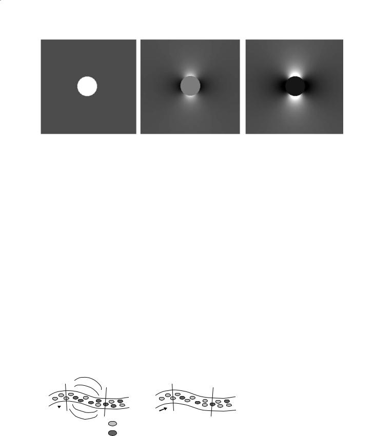
fMRI experiment and enables changes in blood oxygenation level to be detected. This is shown schematically in Fig. 8.3 where the simulated magnetic field is shown for a blood vessel that contains partially deoxygenated blood. Figure 8.3a shows the case of the vessel being aligned with the main static B0 field. In this case there is a shift in the magnetic field within the vessel, but little distortion of the field surrounding the vessel. As the angle between the blood vessel and the main B0 field is altered to 45º (Fig. 8.3b) and 90º (Fig. 8.3c) it can be seen that the intravascular magnetic field is altered, and there is a progressively larger effect outside the blood vessel. In a representative tissue voxel there will be a random distribution of microvascular orientations resulting in a complex field distribution both for the intravascular water spins, and the extravascular (tissue) water spins. These field distributions lead to the T2* shortening that is the origin of the BOLD effect.

In practice both the water molecules in the blood itself (the intravascular compartment) and the water molecules in the tissue space that surrounds the vessels (the extravascular compartment) contribute to the MRI signal that is measured. Since the arte-

rial blood is fully oxygenated under normal circumstances, and since this does not change during periods of neuronal activity, it is only necessary to consider the signal changes that originate within and around the capillary and venous vessels. Various authors have conducted theoretical and numerical calculations which show that the extravascular signal contribution is given by the following formula (Ogawa et al. 1993):

where R2*BOLD is the BOLD relaxation contribution to R2* (=1/T2*), vBmax = 2πγ∆χB0, and CBVv is the

fractional blood volume of capillaries and venules in grey matter. Hence there will be a change in the signal intensity in a T2*-weighted image if either the blood oxygenation term (Y) changes, and/or if

the CBV changes. It is instructive to compare the form of Eq. 2 with the CBV and BOLD plots shown in Fig. 8.2. Note that the increase in CBV during neuronal activation leads to an increase in R2*BOLD (via Eq. 2) and hence to a signal decrease (T2* shortening). However, the increased oxygenation level of the blood (Y) that indirectly results from the increase in

CBF leads to a decrease in R2*BOLD (and hence to a signal increase). As can be seen in Fig. 8.2, these two

effects compete with one another to yield a complex BOLD time-course that may have both positive and negative epochs.

A summary of these effects is shown in Fig. 8.4, demonstrating how shifts in the haemodynamic variables during neuronal stimulation lead to changes in the concentration of deoxyhaemoglobin in the tissue voxel, and hence to a signal change in a T2*-weighted image.

Fig. 8.4. Diagram showing the haemodynamic variables that change during neuronal activity. In the basal state deoxyhaemoglobin in the capillaries and venules causes microscopic field gradients to be established around the blood vessels. This in turn leads to a decreased signal in a gradient-echo MRI sequence. In the activated state the significant increase in flow and modest increase in oxygen demand result in a lower concentration of deoxyhaemoglobin in the capillaries and venules. As a result the field gradients around the vessels are diminished and the gradient echo signal is restored.

Functional MRI

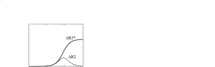
Fig. 8.5. Extravascular ∆R2* and ∆R2 changes versus vessel radius for a gradient-echo sequence (solid line) and SE sequence (dashed line).

Before leaving the topic of BOLD theory it should be pointed out that it is also possible to obtain BOLD sensitivity when using a purely T2-weighted pulse sequence (see also the discussion on T2 contrast below). The reason that the majority of BOLD fMRI studies to date have used pulse sequences that are based on gradient echoes rather than spin echoes can be appreciated by reference to Fig. 8.5.This shows the theoretical effect on the relaxation rate of transverse magnetization (R2=1/T2 for a spin-echo (SE) sequence, and R2*=1/T2* for a gradient-echo (GE) sequence) as a function of the radius of the blood vessels. In both cases the same level of blood deoxygenation has been modelled. It can be seen that the GE sequence (solid line) shows a much larger change in relaxation rate for a given level of deoxygenation than the SE sequence (dashed line), provided the vessel radius is above approximately 8 µm. The origin of this effect lies in the difference in the regimes of characteristic diffusion distances relative to the extent of the field inhomogeneities surrounding vessels of different sizes. Above approximately 8 µm radius the signal dephasing effects of the blood deoxygen- ation-related field inhomogeneities will be substantially refocused by a SE sequence (leading to small R2 changes), but will continue to dephase in the case of a GE sequence (leading to significant R2* changes).A disadvantage of GE sequences can also be observed in Fig. 8.5, however. This is that GE sequences show signal changes even from very large blood vessels that may not be localized to the active tissue – the so-called draining vein effect (Turner 2002). BOLD signal changes can be observed if a SE pulse sequence is employed, but the percentage signal change that is measured is much smaller than in the case of a GE pulse sequence.

97

8.2.3

Other MR-Accessible Markers of Functional Activity

The description above concentrates on the BOLD effect, since this is the contrast mechanism used in most fMRI examinations. However, it is worth mentioning other physiological and biophysical parameters to which MRI can gain access. None of these other contrast mechanisms is used widely, although each has the prospect of revealing additional functional information, and hence may become clinically relevant.

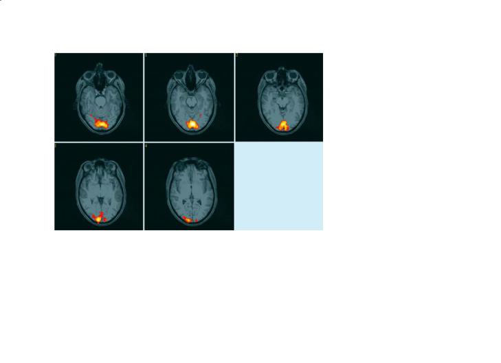
CBF: Probably the most informative of these additional MRI contrast mechanisms is the measure of CBF. As described in the preceding chapter, there are two principal methods for assessing CBF using MRI: either using an exogenous paramagnetic contrast agent (Ostergaard et al. 1996), or by magnetically labelling the arterial blood itself using specialized RF pulses (Williams et al. 1992; Wong et al. 1999). Both of these methods allow resting levels of perfusion to be measured, although both approaches have certain unresolved methodological issues that limit their interpretation in the clinical setting. One advantage of the non-invasive spin labelling approach, though, is that it can be used to measure dynamic changes in blood flow during neurological stimulation (Kim et al. 1997; Luh et al. 2000). These preliminary results also suggest that perfusion contrast is better localized to the parenchymal tissue and less contaminated by artefacts from draining veins than is BOLD contrast. The main disadvantage of arterial spin labelling is that the contrast-to-noise ratio is very low, despite the fact that the underlying regional CBF changes themselves are quite large (30–100%), with sensitivity down by at least a factor of three relative to BOLD contrast. As a consequence, perfusion fMRI is still only performed in a small number of rather specialist research centres. An example of a perfusion time-course and a perfusion activation map is shown in Fig. 8.6.

CBV: Another physiological correlate of functional activity is that of local changes in CBV. Indeed, the first functional MRI methods used the blood volume change as the basis for the fMRI contrast (Belliveau et al. 1991). The CBV response to neuronal activity is thought to be a purely mechanical response of the cerebral vasculature to increases in CBF, and hence pressure (Buxton et al. 1998; Mandeville et al. 1999). MRI methods to measure CBV have used

exogenous contrast agent injection (e.g. gadoliniumbased compounds such as gadopentetate dimeglumine) in order to map blood volume by measuring the passage of a bolus of contrast agent through the tissue of interest (Rosen et al. 1991). In order to show an fMRI response it is necessary to perform two separate bolus injections, one during stimulus condition A and the other during stimulus condition B. CBV changes can then be calculated from the difference in the CBV maps calculated during conditions A and B, after accounting for any normalization issues. Clearly, this method is cumbersome, since it requires invasive injection procedures, and is also limited to comparison of only a very few stimulus conditions (usually only a single comparison of A and B).

An attractive alternative approach uses long-last- ing susceptibility-based exogenous contrast agents that may offer the possibility to map CBV changes dynamically. These iron oxide-based agents have long half lives in the blood (several hours) and so may allow more elaborate CBV-based fMRI to be performed. To date these agents are only permitted for animal use (e.g. Mandeville et al. 1998).

CMRO2: The metabolic rate of consumption of oxygen (CMRO2) is a parameter that is more intimately related to the underlying neuronal activity than either the BOLD or CBF changes. For this reason there have been several attempts to measure CMRO2 using MRI. One approach has recently been proposed by Davis et al. (1998) and by Hoge et al. (1999) that allows a determination of the percentage change in CMRO2 during activation, although it does not allow an absolute quantification of CMRO2. The method requires an independent calibration of the confounding effects of CBV in the BOLD response equation (Eq. 2). Since direct dynamic measurement of CBV using MRI is still not possible in humans, the calibration is accomplished by measuring the dynamic CBF response to hypercapnia and then by using the empirical relationship of Grubb et al. (1974) to infer changes in CBV.

Using this approach, there remain a number of questionable assumptions that are implicit in the determination of CMRO2 change from MRI data. The principal assumption is that Grubb’s equation relating changes in CBF and CBV holds for conditions of

activation, and that it holds in awake humans (the original empirical relationship was established in anaesthetized monkey brain). Another implicit assumption when fitting to the models used to date is

that only the extravascular contribution to R2*BOLD is modelled. As described in the earlier sections above,

this is not strictly true. For now, measurement of CMRO2 change in humans remains very challenging, but may in the future become an important adjunct to fMRI studies, particularly in clinical populations.

T2: There is a long history in the NMR literature of studying the oxygenation dependence of the T2 of blood itself, and indeed debate still exists regarding the precise mechanisms involved in the origin of the phenomenon (Springer 1994; Ye and Allen 1995). Regardless of the mechanism, the T2 value of blood is dependent on a number of parameters in addition to blood oxygenation, including haematocrit, field strength, and echo time (conventional SE sequence) or echo-to-echo spacing (Carr-Purcell-Meiboom-Gill sequence).

Most current theories of blood T2 (e.g. van Zijl et al. 1998) model the oxygenation dependence as an exchange phenomenon between intracellular and extracellular environments. Empirically, the measurements fit well to the equation:

In this equation T2blood is the observed T2 value of the whole blood and T2plasma is the T2 of the plasma compartment alone. T2ery is the T2 of water in the

erythrocytes (red blood cells), which depends on the oxygenation fraction of the haemoglobin. T2exch is the term that accounts for exchange of water between the intracellular compartment (i.e. inside the erythrocyte) and the extracellular compartment (i.e. the plasma). The form of this equation is typical for a system that is in fast exchange on the NMR time scale (TE in this case) – for such a system the relaxation rate that is observed is simply the sum of the rates of contributing relaxation processes.

Theory and experiment show that the term (1/ T2ery) depends linearly on the oxygenation fraction of the haemoglobin, and that the exchange term (1/ T2exch) depends quadratically on the oxygenation fraction of the haemoglobin, as well as being dependent on the individual’s haematocrit. This suggests that blood T2 is able to report on a physiologically meaningful parameter, namely blood oxygenation, if the blood haematocrit can be measured or assumed.

Specifically, as the blood oxygenation increases during neuronal stimulation, the T2 value of blood rises, leading to more NMR signal originating from intravascular water spins. In an attempt to utilize this mechanism, van Zijl and colleagues have developed elaborate procedures for calibrating the terms in Eq. 3 such that the blood oxygenation can be estimated from its measured T2 value (van Zijl et al. 1998). Although accurate vascular T2 measurement is very difficult to perform experimentally, and can only really be accomplished in a large draining vein, values have been derived for the change in oxygen extraction fraction that are consistent with literature values (Oja et al. 1999; Golay et al. 2001).

8.3

Acquisition Practicalities

8.3.1

Pulse Sequence Selection

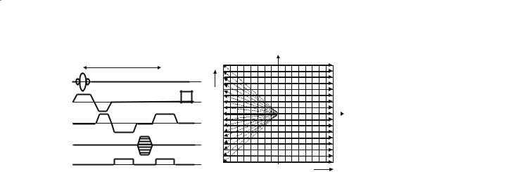
Since the GE signal change in response to a change in blood deoxygenation level is significantly larger than for a SE sequence, GE sequences have been used for the majority of BOLD fMRI studies. There are several available pulse sequences that can be applied to fMRI (only a subset of which are discussed in this section). The decision of which to choose depends on such factors as the capability of the available hardware, requirements for spatial and temporal resolution, and the area of the brain that is under study. A review of some of the most commonly encountered pulse sequences is provided below. For most of the sequences a pulse sequence diagram is shown. This is a timing diagram of the events that occur on the three gradient axes (slice select direction Gsl, read out direction Grd, and phase encode direction Gpe), the radiofrequency pulses (RF), and the data acquisition, controlled by the receiver gate. The purpose of the pulse sequence is to allow the adequate sampling of k-space (see Chapter 4 Fast Imaging in this volume for a discussion of k-space).

FLASH: The FLASH GE sequence (Haase et al. 1986) has been used by several groups who do not have access to fast gradient hardware technology. A pulse sequence diagram for the FLASH sequence is shown in Fig. 8.7, along with a map of the way in which k-space is sampled for this sequence. Note that each repetition of the pulse sequence acquires only one line of k-space, and that N repeats must be ac-

100

TE

RF

Gsl

Grd

Gpe

receive gate

NAV data

quired in order to build up the data for an N×N image. Also known as the SPGR and FFE sequence, the FLASH sequence is a conventional GE technique that requires 3–6 s per slice to acquire the data. For this reason whole-volume studies are impractical using the FLASH approach, although the method does offer the advantage of having only a low sensitivity to geometric distortion (see below). However, because of the lengthy time of acquisition for each FLASH image the technique is very sensitive to small hardware or physiological instabilities.

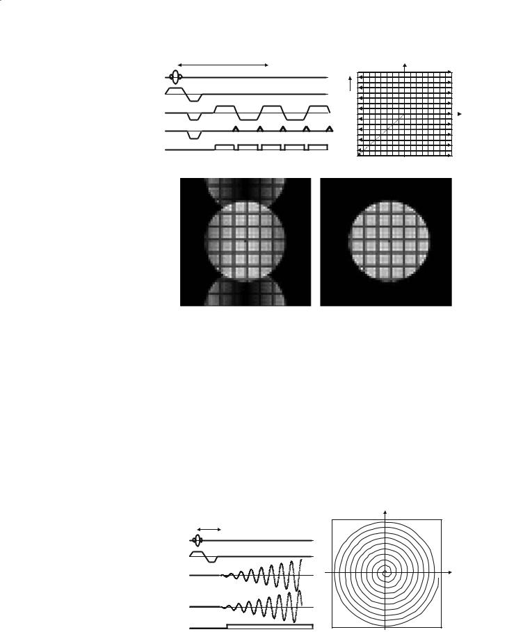
EPI: Echo planar imaging (Mansfield 1977) is the most widely used fMRI pulse sequence due to its remarkable speed of acquisition. On modern scanners the whole head can be covered at 4 mm slice thickness in about 3 s (ten slices per second). This enables the experimenter to characterize the haemodynamic response (the time for local flow increases and decreases to occur in the brain in response to brain activity is on the order of 6–8 s), which can yield additional information. EPI can be used to provide either T2* contrast (GE variant) or T2 contrast (SE variant).

Since EPI is so widely used it will be described in some detail here. A pulse sequence for EPI is shown in Fig. 8.8, along with the corresponding k-space sampling scheme. The principal difference with respect to the FLASH sequence is the ability of EPI to sample the whole of k-space following a single excitation of the slice. Typically, the entire information for an (admittedly low-resolution) image of the slice can be acquired in 40–50 ms. So-called “snap-shot” EPI sequences are limited to acquiring images with a matrix resolution of approximately 64×64 pixels, and on some systems up to 128×128. However, it is possible to use an interleaved version of the basic EPI sequence in which larger image matrix sizes can be achieved (McKinnon 1993). This is at the expense of a decreased temporal resolution, though, since the

data for each slice requires the combination of data from multiple excitations of the slice (typically 4–16 excitations).

The major drawback of EPI, aside from its inherently low spatial resolution (usually about 4×4 mm in plane and 4–6 mm slice thickness), is its sensitivity to a number of sources of artefact. The two most prominent issues are those of non-linear geometric distortion and Nyquist ghosting. Geometric distortion occurs principally in the phase encode direction (Jezzard and Balaban 1995), and makes coregistration between EPI and conventionally collected data sets problematic. It is caused by the misrepresentation in the position of pixels that occurs in regions where the magnetic field homogeneity is poor, principally in the frontal and temporal regions of the brain where inherent susceptibility-based distortions are present in the magnetic field. The other prominent image artefact that is encountered with EPI is the phenomenon of Nyquist ghosting. This occurs as a result of the generation of the image from both positive going (left to right) and negative going (right to left) lines in k-space (see Fig. 8.8). This is in contrast to almost all other MRI pulse sequences in which every line in k-space is collected under the same readout gradient polarity. A number of small imperfections in the scanning process (e.g. scanner hardware imperfections and magnetic field inhomogeneity effects) will lead to a line-to-line modulation in the k-space data that, when Fourier-transformed to produce the final image, leads to some of the image signal being displaced by half a field of view (for snapshot EPI – more complex patterns occur for the case of interleaved EPI). This effect is shown in the lower left panel of Fig. 8.8, demonstrating a prominent “ghost” image that is displaced by half the field of view in the phase encode direction of the image. Various correction algorithms have been developed to minimize this artefact (to form the corrected image shown in the lower right panel of Fig. 8.8), but

in the common situation when the ghost signal impinges on the main image, it is wise to be aware of possible “aliased” fMRI activations that can originate from the ghost and therefore occur half a field of view from their true origin. For example, this has been noted to be a particular problem for “phantom” eye movements (Chen and Zhu 1997).

Spiral: Spiral imaging (Meyer and Macovski 1987) is also increasingly used by fMRI researchers, and is shown in Fig. 8.9. The method is similar to EPI in temporal resolution and in its ability to be run in a GE or SE mode. The artefacts that spiral sequences

generate are different to EPI, yielding a local blurring (deterioration in point spread function) rather than geometric distortion in the presence of field inhomogeneity effects. Spiral sequences are also less demanding on the gradient amplifiers, and have therefore been observed to give improved stability.

PRESTO: The PRESTO sequence (Liu et al. 1993) uses echo shifting principles (Moonen et al. 1992) in order to achieve a short TR time without compromising T2* sensitivity. A conventional phase encoding strategy is used, so geometric distortion is minimal with this sequence. Another benefit is that because

the sequence can be run in a true 3D mode, it can be made very insensitive to unwanted arterial inflow contamination that can confound the FLASH approach (Duyn et al. 1994). A pulse sequence diagram for the PRESTO sequence is shown in Fig. 8.10. The gradient pulses shown hatched in Fig. 8.10 are used in such a way as to ensure that magnetization excited during TR period i is not refocused to form imaging data until the (i+1)th TR period.As such, the TE time is equal to 1.5TR (in the sequence shown). This allows adequate GE weighting to be achieved (to give BOLD T2* contrast), but retains a short TR, allowing 3D images to be acquired in a reasonable time.

Spin-Echo BOLD Sequences: As mentioned above, SE sequences generally demonstrate lower BOLD contrast. However, some researchers have used sequences based on SE pulse sequences, either in order to recover some of the signal lost in frontal and temporal regions of the brain, or to quantitatively measure the T2 relaxation time of blood. In the former case a hybrid sequence that combines GE and SE contrast can be used. This is known as an asymmetric spin echo, and is achieved by introducing an asymmetric delay into an otherwise standard SE sequence.A modification of the standard BURST pulse sequence (Hennig and Hodapp 1993; Lowe and Wysong 1993) is one such example. The sequence uses a train of low flip angle RF excitation pulses in the presence of a readout dephasing gradient. These are subsequently refocused as a train of echoes following a 180° pulse. The method is capable of producing “snap-shot” low-resolution images, and has the added benefit of being very quiet (since very few gradient switches are required). The sequence has been applied to fMRI (Jakob et al. 1998) by use of an asymmetric SE approach that provided the T2* BOLD contrast. The BURST sequence has a much lower signal-to-noise ratio than the EPI sequence, but may have applications where a quiet pulse sequence is required (e.g. for auditory activation studies).

8.3.2

Scanner Hardware Requirements

In order to accomplish successful fMRI a scanner that is above all stable and that also offers good sig- nal-to-noise ratio is essential. Further, fast gradient hardware is desirable, since rapid sequences such as EPI provide an increase in the number of independent samples of brain activity, and hence improved statistical confidence in the resulting fMRI maps. Considerations include:

Magnetic Field Strength: Implied within the BOLD equation (Eq. 2) is a dependence of the BOLD relaxation rate that is linear with static magnetic field strength. This is in practice what is observed, although there are a number of qualifying statements to be made. Firstly, Eq. 2 only considers the extravascular spin contribution and,indeed,only for spins surrounding those vessels with a radius above approximately 10 µm. In the case of smaller vessels, and in the case of SE weighted sequences, even higher order dependencies are predicted, making higher field strength all the more attractive. Working against high field, however, is the shorter inherent T2* of the tissue. This attenuates the effect of the change in R2* (i.e., T2*) that accompanies neuronal activation, but has the advantage of suppressing large vein signals. Experimental assessment of these issues indicates that higher field strengths are indeed beneficial (Gati et al. 1997), despite a greater contribution of physiological noise at high field (Kruger and Glover 2001). As a practical guide, a field strength of between 1.5 and 3 T should provide adequate fMRI sensitivity. It should be noted that at very high field (4 T and greater) one encounters increasingly severe RF field homogeneity problems, and severe magnetic susceptibility problems.

Gradient Performance: Fast gradient performance is highly desirable for fMRI studies allowing fast imaging sequences, such as EPI, to be performed.

Practically, one needs gradient strengths of the order 25 mT/m and gradient slew rates of 150 T/m/s. Lower performance figures than this will perhaps suffice, but fast imaging sequences may become impractical if performance is substantially lower than the above. Related to gradient performance is fast data acquisition and processing capability. As a benchmark figure, a sustainable acquisition rate of ten frames per second in snap-shot EPI mode is desirable.

Stability Requirements: Since fMRI is a subtle effect (0.5–5% signal change typically), it is important to optimize the experiment as much as possible. One critical factor is to ensure that the MRI system hardware is of sufficient signal-to-noise ratio and stability over time that an effect on the order of 0.5% can be detected.It is therefore important to run regular quality assurance tests using a phantom sample that loads the coil in a similar way to the human head. Such data will reveal whether the system has stability problems that should be addressed before fMRI experiments are attempted. A recommended test that can be performed is a pseudo-fMRI experiment in which a phantom sample (e.g. a spherical agar gel phantom) is imaged using an otherwise standard fMRI protocol. One example would be an EPI time-course consisting of 100 volumes, 64×64 pixels, 25 slices, TR/TE/thk=3000 ms/40 ms/5 mm, FOV=24×24 cm. A number of tests can then be performed on each slice of the data, including:

1)Mean signal variability: Variability in the timecourse of the mean signal from the central 80% of the image. This figure should reflect the transmitter stability and be better than 0.1%.

2)Signal-to-noise ratio of the individual images: Signal = mean of central 20% of phantom, Noise = standard deviation of non-ghosted noise region. Ideally the ratio should be more than 250. (Note that a true signal-to-noise measure requires a correction factor of 1.53 (Weisskoff 1996) to account for the Rician nature of noise in magnitude MRI data.)

3)Level of EPI ghost: For EPI sequences the ghost should be <2–3% of the main image intensity.

4)Pixel-by-pixel temporal stability: For each pixel the temporal standard deviation in intensity is calculated. This is expressed as a percentage of the image mean intensity and should be <0.5%.

5)Spatial drift test: A data registration test is useful to assess the drift of the image in the field-of-view throughout the scan. This test can report on problematic gradient coil heating or other instabilities

leading to drifts in the B0 field. The test is best done on the volume data.

8.3.3

The Scanner as a Psychophysical Testing Environment

A key difference between conventional MRI scanning and fMRI is the need for external stimuli to be presented to the subject in the scanner and for response recording to be made from the subject. One principal requirement is the addition of a method of visual stimulus presentation (although many clinical MRI scanners now come equipped with a suitable device designed to minimize patient anxiety).This presentation device needs to be under computer control, and ideally should be capable of being triggered from the scanner. Finally, a comprehensive software package must be provided to control stimulus presentation and scanner synchronization of all stimulus and response events.

8.4

Experimental Design

8.4.1

Block Design Paradigms

The simplest form of fMRI paradigm that can be conducted is known as the block design. This is shown in Fig. 8.11a and consists of blocks of time when the stimulus is present (shown shaded) and blocks of time that act as a control periods. Typically a sustained period of at least 20–30 s forms each stimulus or control period. In some circumstances it is sufficient to use“rest”as the control condition (i.e. subject lying in the scanner “doing nothing”). However, this is a very uncontrolled condition, and often leads to difficulties in interpretation. In such circumstances, it may be necessary to select a control task that replicates many of the stimulus inputs present in the task condition, but excludes a single specific aspect that is the functional processing unit of interest. In addition to the single task period shown in Fig. 8.11a, it is also possible to design paradigms that probe several functional attributes, even in parallel. Such an example is shown in Fig. 8.12 which displays the results of overlapping periods of visual and auditory stimulation, each having a different time course. When analysing the data,the two different time series “signatures” of the visual and auditory stimuli lead to distinguishable activation areas in the brain (coloured yellow–red and green–blue, respectively).