Книги по МРТ КТ на английском языке / MR Imaging in White Matter Diseases of the Brain and Spinal Cord - K Sartor Massimo Filippi Nicola De Stefano Vincent Dou

Mark A. Horsfield

CONTENTS

1.1.1Nuclear Magnetism 3

1.1.2Precession 4

1.2.1Overview 7

1.2.3T2-Weighted Imaging 9

1.2.4T2*-Weighted Imaging 10

1.2.5T1-Weighted Imaging 10

1.2.6 Summary of Simple MRI Contrast 12

1.1

The Magnetic Resonance Signal

1.1.1

Nuclear Magnetism

In the materials that we traditionally think of as being magnetic (such as iron and steel), the magnetism arises from two properties of electrons: charge (all electrons are negatively charged) and motion (electrons rotate or spin about their axis).A moving charge will always generate a magnetic field, and in this way an electrical current flowing through a wire generates a magnetic field around the wire. While a single rotating electron generates a magnetic field,electrons tend to form themselves into pairs, with one electron rotating in one direction and the other electron rotating in the opposite direction. The magnetic field of one electron cancels out the field from the second, and the net magnetism of the pair is zero. In materials with unpaired electron spin, the magnetic field from individual electrons may be randomly aligned,

M. A. Horsfield, PhD

Department of Cardiovascular Sciences,University of Leicester,

Leicester, LE1 5WW, UK

so that under these circumstances the net field from the material will be zero. However, if such a material is brought into a magnetic field (the applied magnetic field), this causes a partial alignment of the electrons’ magnetic fields and the material becomes slightly, and temporarily magnetized. These types of material are called paramagnetic.

We do not usually think of people as being magnetic, and indeed some of the principal constituents of the human body (e.g., water, lipids, proteins) do not show any magnetic effects from their electronic structure. However, another, weaker form of magnetism (nuclear paramagnetism) arises from the charge and spin of nuclear particles in just a few types of nuclei, where the spin of individual protons and neutrons is not canceled out within a nucleus.Table 1.1 shows a list of some of the most interesting nuclei (from a biological point of view) that exhibit nuclear magnetism.

Table 1.1. Biologically interesting nuclei that give an MRI signal

aRelative sensitivity indicates the amount of signal (compared to hydrogen) and is for equal numbers of atoms per unit volume of tissue. The relative sensitivity takes into account both the Larmor frequency and the natural abundance of the given isotope.

The hydrogen atom is most commonly used when performing MRI scanning, since the hydrogen nucleus gives the strongest signal, and there is plenty of hydrogen around in the human body in molecules of water, fat and proteins. Potentially, other nuclei could be used, but the poor sensitivity would make for very poor quality images, and excessively long scan times.

4

1.1.2 Precession

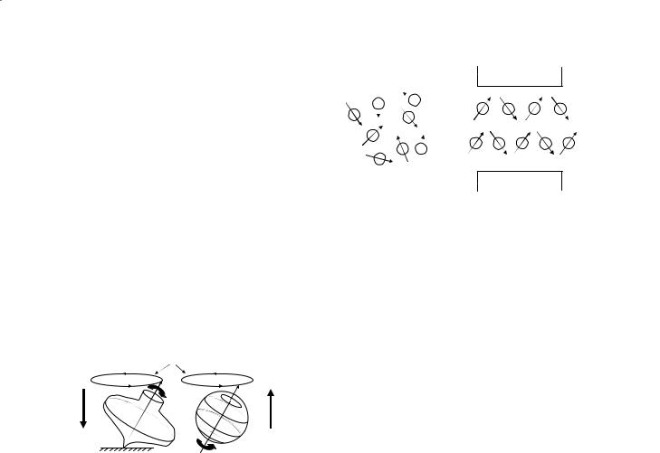
The hydrogen nucleus spins about its axis, generating the nuclear magnetism, but when the nucleus is placed in a magnetic field, it undergoes another form of rotary motion called precession. This type of motion can also be seen with a child’s spinning top if it is tilted at an angle to the gravitational field.

The frequency of this precessional motion is called the Larmor frequency, and is proportional to the applied magnetic field strength:

In the Larmor equation, above, γ is the gyromagnetic ratio and is constant for all nuclei of the same type, but varies between different types, as shown in Table 1.1.

Precessional motion

Fig. 1.1. The angular momentum of a spinning top (left) interacts with the gravitational field to produce a rotary “precessional” motion. In a similar way, the magnetism of the nucleus (right) interacts with the applied B0 field to cause precession about the field

1.1.3

Polarization and Coherence

Since nuclear magnetism is a form of paramagnetism, the individual nuclear spins do not have any preferred alignment until they are placed in the applied field (the B0 field). A large component of any MRI scanner is the magnet in which the patient lies, which causes the nuclear spins to become aligned, or polarized, such that some spins point in the general direction of the applied field, and some point in a direction opposed to the applied field.

There are slightly more spins aligned with the applied magnetic field than there are opposed to it,although the difference in the numbers is very small. This difference is the excess population of spins. Now, when the magnetism of the individual spins is added together, the net result is a small amount of magnetization in the same direction as the applied field that arises within the patient. The amount of this net magnetization is propor-

M. A. Horsfield

N

S

Fig. 1.2. When no magnetic field is applied (left), nuclear spins have no preferred alignment so that the net magnetization within the patient is zero. When a magnetic field is applied (right), polarization occurs with some spins being aligned with the field, and some opposed to it. There are slightly more spins aligned with the field than opposed, giving rise to magnetism within the patient – the “net magnetization”

tional to the strength of the applied field,hence the need for a powerful magnet at the heart of the MRI scanner. However, because the net magnetization points in the same direction as the applied field and is much, much smaller than it,it is very difficult to measure directly.We need to tilt the patient’s magnetization away from the applied field in order to make it measurable.

1.1.3.1

Radio Frequency Pulses

The patient’s net magnetization is made measurable by applying a burst (pulse) of electromagnetic energy. The transfer of energy from the electromagnetic wave to the nuclear magnetization is a resonance phenomenon, meaning that the frequency of the pulse must be close the spins’ natural frequency (the Larmor frequency) in order to have the desired effect. Since the Larmor frequency is in the radio frequency range (MHz), then the pulse is called a radio frequency (RF) pulse.

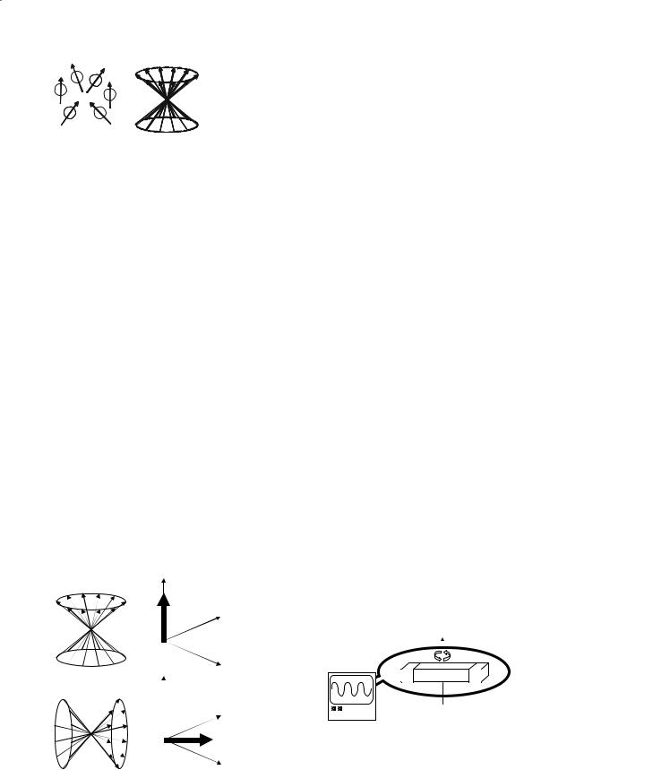
Before the RF pulse is applied, the patient’s net magnetization is usually shown schematically as in Fig. 1.3. Note that: (a) only the excess population of spins is shown, and (b) although no individual spin is aligned with the B0 field, the net result of adding all these spins together is a net magnetization that points in the direction of that field. Since the patient’s magnetization has a direction as well as a magnitude, it is a vector quantity called the net magnetization vector, and given the symbol M. The magnitude of M when the patient has become fully magnetized is given the symbol M0, and depends on the strength of the B0 field and the number of hydrogen atoms per unit volume of tissue that contribute to the magnetization vector. An RF pulse tilts this vector out of alignment with the B0 field, and the angle of tilt (or

M0

Fig. 1.3a–c. Three different ways of representing the patient’s magnetization. a The excess population of spins that (by definition) tend to be aligned with the applied field. b A schematic representation of these spins, indicating that the component of magnetization perpendicular to B0 is random, such that any transverse components of magnetization cancel to zero. c The resultant magnetization vector after adding the individual nuclear magnets together. This net magnetization vector also points in the same direction as the applied field, and is therefore difficult to detect directly

the flip angle) depends on the strength and duration of the RF pulse. When one or more RF pulses is applied, and the MRI signal is measured (see below), then this is called a pulse sequence.

1.1.3.2

90° Pulse – Excitation and FID

A 90° pulse will tilt the net magnetization vector by 90°. If M starts off aligned with the B0 field (by definition, the z direction), then a 90° pulse flips the magnetization into the x-y plane (see Fig. 1.4).

M then precesses in the x-y plane so that, in effect, we now have the patient’s magnetization rotating in a plane perpendicular to the applied field. The method of detecting M is analogous to a motor car’s alternator which generates electricity to power the ignition, lights etc. An alternator consists of a magnet inside some coils of wire, with the magnet being driven by the motor to that it rotates inside the coils.This gener-

z

y

M0

x

az

M0 y

M0

x

b

Fig. 1.4a,b. Individual spins (left) and the net magnetization vector (right) (a) before (a) and just after (b) a 90° RF pulse. The vector has been tilted out of alignment with the B0 field and into the x-y plane

ates an electromotive force (voltage) within the coils. Similarly, we wrap a coil of wire around the patient (the receiver coil) and can measure an oscillating voltage across the coil, with the frequency of oscillation being equal to the Larmor frequency, and the size of the voltage being dependent on the number of hydrogen nuclei that are within the coil.

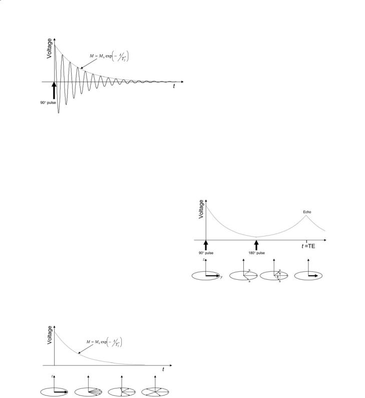
While the magnetization remains in the x-y plane, and the individual nuclear spins are oriented in the same direction as shown in Fig. 1.4 (i.e., they are coherent), a voltage will be measured in the coil. However, there are slight, natural variations in the Larmor frequency due to the interactions between magnetic particles (such as the nuclei) within the patient, and these variations in frequency cause the signal to die away (the magnetization loses coherence) normally within the course of a few hundred milliseconds or so. The initial voltage and its subsequent decay are known as the free induction decay (FID), since the voltage is produced by electromagnetic induction, and once M is in the x-y plane it can rotate freely without further influence from RF pulses.

After application of the 90° RF pulse, the voltage measured in the receiver coil that is wrapped around the patient takes the form of a sinusoidal oscillation with decaying amplitude.The“envelope”that encloses the FID, shown as a dotted line in Fig. 1.6, indicates the rate at which the sinusoid decays, and the time constant that characterizes the decay is called T2* (“T2 star”). T2* depends on both the physico-chemi- cal properties of the tissue and on the uniformity, or homogeneity, of the applied magnetic field. Tissues that have a high free water content tend to have longer T2* values than tissues with a dense matrix of cell membranes and cellular structures. Thus, T2* can be used as the basis for imaging many pathological tissues such as MS lesions, since the density of these cell membranes and structures is reduced by processes such as demyelination and axonal loss, leading to in-

Fig. 1.5. A voltage will be induced across the ends of a coil of wire placed around a rotating magnet. In an MRI scanner, this rotating magnetism originates in the patient after a 90° pulse has been applied. An oscilloscope connected to the coil would show a sinusoidally oscillating voltage, with the frequency of oscillation equal to the Larmor frequency, and the peak-to- peak voltage being proportional to the number of spins within the sensitive region of the coil

Fig. 1.6. A 90° pulse of RF energy tilts the magnetization vector into the x-y plane where it generates an oscillating voltage in the receiver coil. The amplitude of this voltage decays with a time constant T2*

creased T2*.The process of generating image contrast will be described more fully later in this chapter.

As mentioned above, T2* decay contains contributions from both the physico-chemical properties of the tissue, and magnetic field inhomogeneities within the patient. These inhomogeneities may result either from imperfections in the design and manufacture of the magnet,or from the magnetic properties of the patient.Any variations in the tissue’s magnetic properties within the patient will result in small but important perturbations in the magnetic field uniformity; these sorts of variation occur, for example, around the interface between the brain tissue and frontal sinuses.It can be seen from the Larmor equation that any variation in B0 field strength will lead to different precessional frequencies throughout the patient, so that the initial magnetization vector, being composed of magnetization from different parts of the patient, will begin to spread out (or‘dephase’) in the x-y plane.This is mechanism by which the FID signal decays after it is initially generated by the 90° pulse (Fig. 1.7).

1.1.3.3

180° Pulse – Refocusing

The initial 90° pulse rotates the magnetization which is initially along the z-axis (longitudinal magnetization) down into the x-y plane and generates the measurable or transverse magnetization. Similarly, a 180° pulse rotates the magnetization vectors by 180°, and one use of these pulses is to reverse the dephasing that occurs after a 90° pulse because of the variations in the B0 field.

Shown in Fig. 1.8 are two packets of magnetization, labeled a and b, with a rotating clockwise (relative to the average) because it experiences a higher B0 field than average (and hence has a higher precession frequency), and b rotating anticlockwise because it experiences a lower B0 field than average. Deviations from the average motion are shown, so that superimposed on this dephasing is a precession at the average

Fig. 1.8. After the initial 90° pulse, dephasing of transverse magnetization occurs, with the magnetization from two locations within the patient, labeled a and b, being shown. A 180° pulse is applied and rotates the magnetization about the y-axis so that the magnetization is flipped over, reversing the phase of a and b. The magnetization continues to precess and comes back into phase at a time TE called the echo time. Deviations from the average motion are shown, so that superimposed on this is a precession at the average Larmor frequency

Fig. 1.7. After the 90° pulse creates magnetization in the x-y plane, variations in the Larmor frequency within the patient will cause a spreading out, since some magnetization precesses slower, and some faster than the average. This spreading out in the x-y plane results in a reduction in the size of the net magnetization vector and is the cause of the decay in the voltage measured in the receiver coil. Deviations from the average motion are shown, so that superimposed on this spreading out is a precession at the average Larmor frequency

Larmor frequency. A 180° pulse will rotate the magnetization about the y-axis, which has the effect of reversing the phase that accumulated before this pulse. After the 180° pulse, a continues to rotate clockwise and b anticlockwise and eventually at a time called the echo time, or TE, the individual magnetization vectors come back into phase generating again a high voltage in the receiver coil.This spin-echo is what is commonly measured during an MRI scanning sequence.

Notice that the voltage in the receiver coil is somewhat reduced in amplitude compared to the initial amplitude after the 90° pulse. That is because the loss of signal due to T2* relaxation has two causes,

and only one of these (the magnetic field inhomogeneities) can be reversed by the 180° pulse. A second cause of signal dephasing is the interactions that occur on a microscopic scale between magnetic entities such as unpaired electrons and other nuclear magnetism within the patient.

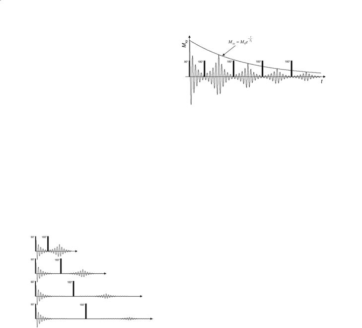
Notice also that the echo forms at a time exactly twice that between the 90° pulse and the 180° pulse. If the time between the 90° and 180° pulses is varied, then TE will also vary and the amplitude of the echo will change, as shown in Fig. 1.9. Because the effects of magnetic field inhomogeneity are removed in the process of forming the echo,then the decrease in echo amplitude as TE increases is due only to the microscopic interactions between magnetic particles within the tissue. These interactions are fundamentally related to the physico-chemical properties of the tissue, and not to the vagaries of the uniformity of the magnetic field.The decay of the echo amplitude shown in Fig.1.9 is exponential with TE and has a time constant called T2, the transverse relaxation time. T2 is also called the spin--spin relaxation time, since the loss of transverse magnetization in this way results largely from interactions between the magnetism of individual spins.

Fig. 1.9. Increasing the time between the 90º and 180º pulses causes the spin-echo to form later. While the effects of magnetic field inhomogeneity are reversed by the 180º pulse, some reduction in the echo amplitude with increasing echo time remains; the time constant for echo amplitude decay is T2, the transverse relaxation time

After the echo is formed, the magnetization again begins to decay because of the magnetic field inhomogeneities. Multiple echoes can be created by applying a series of 180º pulses. The echoes form between the pulses, and these multiple echoes are called the echo train. In this way, the MRI signal can be measured more than once, since each echo gives us a measurement. The envelope that encloses the peaks of the echoes in the train is also an exponential decay with time constant T2 (Fig. 1.10).

Fig. 1.10. Multiple spin-echoes are formed by applying 180º pulses in succession. The echoes form in the spaces between the pulses, and the amplitude of echoes in the “train” decreases exponentially with a time constant T2

1.2

Relaxation and Image Contrast

1.2.1 Overview

The above has provided the background needed to understand the nature of the MRI signal, how that signal is generated and how it decays due to transverse relaxation (T2*). The following will give more detail about how these processes can be used to create MR images with contrast that helps in the diagnosis and characterization of disease. The brightness of any tissue in an MR image is fundamentally related to the number of hydrogen atoms (or nuclear spins) per unit volume of that tissue since this determines the voltage that is generated in the receiver coil by magnetic induction. However, we can exploit the relaxation characteristics to modulate that brightness according to the physico-chemical properties of the tissue; these properties are different for different tissue types, and for tissue affected by disease.

1.2.2

The Bloch Equations

The nuclear spins exist in equilibrium with their surroundings. At equilibrium, the magnetization within the patient is aligned with B0 field (defined as the longitudinal direction, or z direction) as illustrated in Fig. 1.3. An RF pulse disturbs the spins from this equilibrium, for example by tilting the net magnetization vector into the x-y, or transverse, plane as shown in Fig. 1.4. The Bloch equations, formulated by Felix Bloch in 1946, describe the return of magnetization to equilibrium after such a disturbance.

8

1.2.2.1

Longitudinal Bloch Equation

This is a differential equation that describes the return of the longitudinal component of magnetization (Mz) to equilibrium:

M. A. Horsfield

Each of these particular forms is of interest in MRI, since both 90° and 180° pulses are commonly applied, and contrast is affected via the longitudinal magnetization.

1.2.2.2Transverse Bloch Equation

b

M0

t

180° pulse

-M0

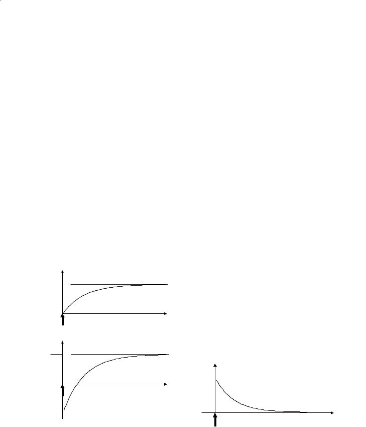
Fig. 1.11a,b. Two particular solutions to the longitudinal Bloch equation. Before an RF pulse is applied, Mz is at its equilibrium value M0. aA 90º pulse tilts the z magnetization into the x-y plane so that Mz=0 at t=0 before it recovers exponentially back to equilibrium.(b)A 180º pulse inverts the z magnetization so that Mz=– M0 at t=0 before again it recovers exponentially to equilibrium

Mxy

M0

t

90° pulse

Fig. 1.12. The solution to the transverse Bloch equation when a 90º pulse is applied, converting all z magnetization to transverse magnetization so that Mxy=M0 at t=0. Mxy decays exponentially to its equilibrium value of zero

1.2.3T2-Weighted Imaging

T2-weighted imaging creates image contrast (differences in tissue brightness) that depends on variations in T2. T2-weighted imaging is simpler to understand than T1-weighting, and is therefore discussed first.

After a 90° pulse, the magnetization lies in the x- y plane and generates the maximum voltage in the receiver coil. This voltage first dies away and then, if a 180° pulse is applied, reforms as an echo at a time TE (Fig. 1.8). The amplitude of the echo depends only on the T2 of the tissue, which in turn reflects the physico-chemical properties of that tissue.

Figure 1.13 shows transverse relaxation curves for two tissues with different T2 values: tissue ‘a’ has the longer T2 and could represent an MS lesion, while tissue ‘b’ could represent normal tissue. An echo time

Signal

can be chosen so that the difference in signal generated by the two tissues,and therefore the difference in brightness, is maximized. When TE is chosen in this way to give contrast, this is known as T2-weighted imaging.

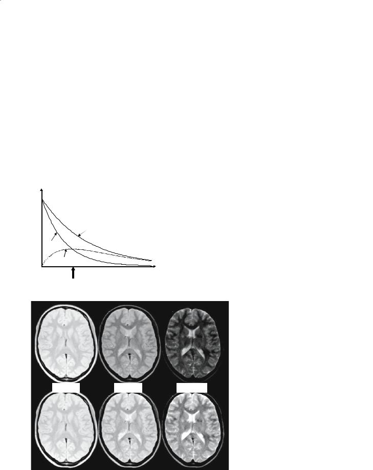
Figure 1.14 shows an axial section of a normal brain, cutting through the lateral ventricles. The same section is shown with three different echo times: 15 ms, 50 ms and 100 ms. Notice that in the top row of images, where the display brightness settings have been kept fixed, the brightness of all tissues decreases with increasing TE, as expected from Fig. 1.12. In the bottom row of images, adjustments have been made to the display brightness setting, as would normally be done, giving the illusion that the signal from some tissues increases with increasing TE.

Contrast = ‘a’-‘b’

Optimal TE

10

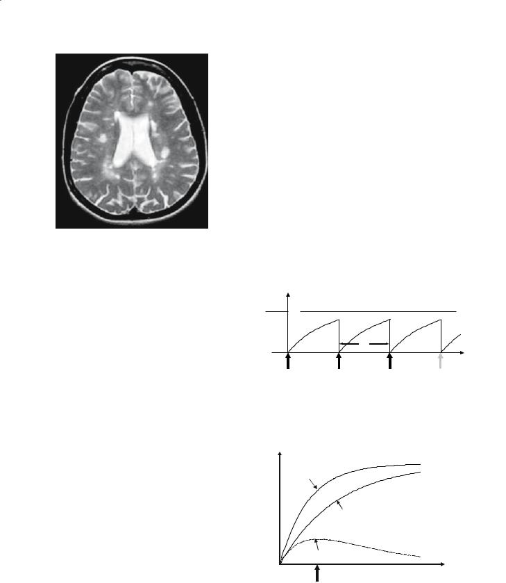
Fig. 1.15. Axial T2-weighted spin-echo image (TE=90 ms) of a patient with multiple sclerosis. Multiple lesions can be seen, particularly around the lateral ventricles, and they are hyperintense because of both their longer T2 and increased proton density

Figure 1.15 shows a typical application of T2weighted imaging in multiple sclerosis. The echo time has been chosen to give good contrast between normal white matter and the MS lesions, which have an elevated T2 and therefore appear hyperintense on this image.

1.2.4

T2*-Weighted Imaging

T2*-weighted imaging employs the same concept as T2 weighting in that there is a delay between the generation of transverse magnetization and its measurement. The difference is that in a T2*-weighted sequence, no 180° refocusing pulse is used, so that the signal decays partly because of magnetic field inhomogeneities with a time constant T2*. This type of scan is sometimes known as a gradient-echo sequence, or sometimes as a FLASH sequence (an acronym for fast low-angle shot).

1.2.5

T1-Weighted Imaging

Longitudinal magnetization is not directly measured by MRI: to generate a voltage in the receiver coil, this longitudinal magnetization must first be tilted into the x-y plane. However, if multiple RF pulses are to be applied, then longitudinal relaxation affects the

M. A. Horsfield

amount of longitudinal magnetization that is available for tilting when the next pulse is applied.

Consider a sequence of 90° pulses applied in succession, with a time between pulses of TR (the repetition time) as shown in Fig. 1.16. Each pulse tilts the z-magnetization down into the x-y plane, generating a measurable signal. Between the pulses, Mz recovers according to the curve described by Eq. (3), so at a given TR, different degrees of recovery of the longitudinal magnetization in different tissues produce contrast according to the T1 of these tissues, as illustrated in Fig. 1.17. Remember that the next 90° pulse converts this recovered longitudinal magnetization into measurable signal, so the T1 indirectly affects the amplitude of the signal and therefore the brightness of that tissue in the MR image. Notice that this is only true for signal generated by the second and subsequent pulses, since the amplitude of the signal after the first pulse is independent of the T1; this first signal is usually discarded.

Mz

M0

TR

t

Fig. 1.16. To collect data for an MR image, a series of 90° RF pulses must be applied, with a separation between each pulse of TR. The amount of longitudinal magnetization before each pulse determines how much signal that pulse will generate. Hence, T1 influences the signal intensity in the image as TR is shortened

Tissue ‘b’

Contrast = ‘a’-‘b’

TR

Optimal TR

Fig. 1.17. Longitudinal relaxation curves for two tissues ‘a’ and ‘b’, with the difference between ‘a’ and ‘b’ shown as the lower dotted curve. This difference is the contrast between the two tissues, and is maximized by judicious choice of TR in T1-weighted imaging

A repetition time can be chosen so that the difference in signal generated by the two tissues, and therefore the difference in brightness, is maximized (see Fig. 1.17). When TR is chosen in this way to give contrast, this is known as T1-weighted imaging.

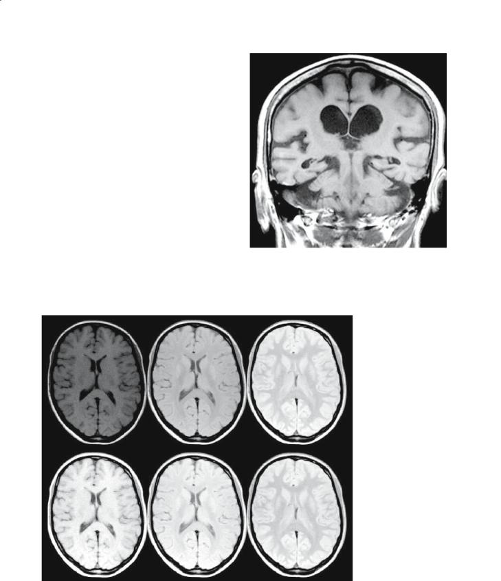
Figure 1.18 shows a normal brain, with three different repetition times: 600 ms, 1500 ms and 4000 ms. In the top row of images,where the display brightness settings have been kept fixed, the brightness of all tissues decreases as TR is reduced, in line with Fig. 1.11. In the bottom row of images, where adjustments have been made to the display brightness settings, there is the illusion that the signal from some tissues increases with decreasing TR.

T1-weighted imaging is typically used in the head to delineate parenchyma from CSF, and is most frequently used to show tissue hypoplasia or atrophy. Figure 1.19 shows a routine T1-weighted scan typical of those used to answer many clinical questions. The TR on this type of scan is chosen to give high contrast between gray matter and CSF, giving good definition of the outline of the brain structures.

Fig. 1.19. A T1-weighted coronal section through the temporal lobes and lateral ventricles of a female (age 79 years) presenting to memory clinic, showing general atrophy of the brain