Книги по МРТ КТ на английском языке / MR Imaging in White Matter Diseases of the Brain and Spinal Cord - K Sartor Massimo Filippi Nicola De Stefano Vincent Dou

1.2.6

Summary of Simple MRI Contrast

The basic factor determining the brightness of a tissue is the number of hydrogen atoms, or protons, per unit volume of tissue, since the signal intensity after an RF pulse is proportional to the proton density in a scan with a long TR and a short TE. Weighting by the relaxation times can be introduced either by shorter repetition time (TR) to give T1 weighting, or by longer echo time (TE) to give T2 weighting. This is summarized and illustrated in Fig. 1.20.

Using a combination of short TR and long TE is not generally useful, since the short TR serves to darken tissues with long relaxation times, while long TE darkens tissues with short relaxation times. Thus, the brightness of all tissues is generally depressed and the resulting image has low intensity and poor contrast (Fig. 1.20).

In biological tissues, it is a general rule that T1 and T2 vary in concert: if T1 is long for a particular tissue, then T2 will also be long, and vice versa. However, there is no strict relationship between them, and the only approximate rule is that the more solid a tissue, or the higher the content of large molecules such as

proteins, and lipids in cell membranes then the lower will be both T1 and T2.

An MRI examination will normally comprise more than one imaging pulse sequence. In the CNS, T1weighted sequences are typically used to show gross anatomy, since the nervous system tissue is shown in relief against a background of dark CSF. Because of this, T1-weighted imaging is sometimes referred to as “anatomical scanning.” T2-weighted sequences are normally used to show changes in tissue that are brought about by disease, since the relaxation times are invariably lengthened in damaged tissue and this shows as a bright region. T2-weighted scanning is sometimes referred to as “imaging pathology.”

This chapter has aimed to provide a basic understanding of MRI. As with many complex subjects, it is necessary in an introduction to gloss over some important issues and leave questions unanswered. For example, the MR image has been mentioned in very abstract terms, with no detail about how we convert the voltage measured in the receiver coil into an image that is shown on the radiographic film or computer display. More in-depth treatment of specific techniques and pulse sequences is given in later chapters.

Short TE

Long TE

Fig. 1.20. Summary of relaxation time weighting of MR images. The fundamental brightness is determined by the number of hydrogen atoms per unit volume of tissue (proton density). Decreasing the TR introduces T1 weighting, and increasing the TE introduces T2 weighting. A combination of short TR and long TE causes a decrease in intensity for all tissues, giving low signal intensity and little contrast

CONTENTS

2.1Introduction 13

2.2Magnets 13

2.2.1Permanent Magnets 14

2.2.2Resistive Electromagnets 14

2.2.3Superconducting Electromagnets 15

2.2.4.2Magnetic Field Strength and Susceptibility Effects 17

2.2.6Field Stability 19

2.3.2Gradient Linearity 23

2.3.3 Gradient Switching and Eddy Currents 23

2.3.4Gradient Strength 24

2.3.5 Gradient Stability and Duty Cycle 24

2.4Radio-Frequency Coils 24

2.5Transmitters 27

2.6Radio-Frequency Receiver 28

K. W. Fishbein, PhD

Facility Manager, Nuclear Magnetic Resonance Unit, National Institutes of Health, National Institute on Aging, Intramural Research Program, GRC 4D-08, 5600 Nathan Shock Drive, Baltimore, MD 21224, USA

J. C. McGowan, PhD

Associate Professor of Electrical Engineering, Department of Electrical Engineering, Murray Hall 227, United States Naval Academy, Annapolis, MD 21402-5025, USA

R. G. Spencer, MD, PhD

Chief, Nuclear Magnetic Resonance Unit, National Institutes of Health, National Institute on Aging, Intramural Research Program, GRC 4D-08, 5600 Nathan Shock Drive, Baltimore, MD 21224, USA

2.1 Introduction

While modern magnetic resonance imaging (MRI) instruments vary considerably in design and specifications, all MRI scanners include several essential components. First, in order to create net nuclear spin magnetization in the subject to be scanned, a polarizing magnetic field is required. This main magnetic field is generally constant in time and space and may be provided by a variety of magnets. Once net nuclear spin magnetization is present, this magnetization may be manipulated by applying a variety of secondary magnetic fields with specific time and/or spatial dependence. These may generally be classified into gradients, which introduce defined spatial variations in the polarizing magnetic field, B0, and radio frequency (RF) irradiation, which provides the B1 magnetic field needed to generate observable, transverse nuclear spin magnetization. B0 gradients are generally created by applying an electric current supplied by gradient amplifiers to a set of electromagnetic coil windings within the main magnetic field. Similarly, RF irradiation is applied to the subject by one or more antennas or transmitter coils connected to a set of synthesizers, attenuators and amplifiers known collectively as a transmitter. Under the influence of the main magnetic field, the field gradients and RF irradiation, the nuclear spins within the subject induce a weak RF signal in one or more receiver coils which is then amplified, filtered and digitized by the receiver. Finally, the digitized signal is displayed and processed by the scanner’s host computer. In this chapter, we will discuss the various technologies currently in use for these components with an emphasis on critical specifications and the impact that these have on the instrument’s performance in specific MRI experiments. While the focus of the current work is imaging, the hardware components described below are also applicable to magnetic resonance spectroscopy (MRS) and this text will include specific information related to spectroscopy where appropriate.

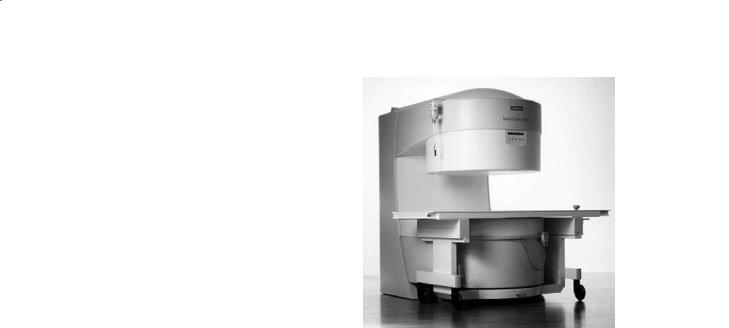
Fig. 2.1. A superconducting clinical magnet system. (Courtesy of Siemens)

2.2 Magnets

The function of a MRI scanner’s magnet is to generate a strong, stable, spatially uniform polarizing magnetic field within a defined working volume. Accordingly, the most important specifications for a MRI magnet are field strength, field stability, spatial homogeneity and the dimensions and orientation of the working volume. In addition to these, specifications such as weight, stray field dimensions, overall bore length and startup and operating costs play an important role in selecting and installing a MRI magnet. Magnet types used in MRI may be classified into three categories: permanent, resistive and superconducting. As we shall see, the available magnet technologies generally offer a compromise between various specifications so that the optimum choice of magnet design will depend upon the demands of the clinical applications anticipated and the MRI experiments to be performed.

2.2.1

Permanent Magnets

Permanent magnets for MRI are composed of one or more pieces of iron or magnetizable alloy carefully formed into a shape designed to establish a homogeneous magnetic field over the region to be

scanned. These magnets may provide open access to the patient or may be constructed in the traditional, “closed” cylindrical geometry. With care, permanent magnets can be constructed with good spatial homogeneity, but they are susceptible to temporal changes in field strength and homogeneity caused by changes in magnet temperature. The maximum field strength possible for a permanent magnet depends upon the ferromagnetic alloy used to build it, but is generally limited to approximately 0.3 T. The weight of a permanent MRI magnet also depends upon the choice of magnetic material but is generally very high. As an example, a 0.2-T whole-body magnet constructed from iron might weigh 25 tons while the weight of a similar magnet built from a neodymium alloy could be 5 tons.While the field strength of permanent magnets is limited and their weight is high, they consume no electric power, dissipate no heat, and are very stable. Consequently, once installed, permanent magnets are inexpensive to maintain.

2.2.2

Resistive Electromagnets

Other than permanent magnets, all MRI magnets are electromagnets, generating their field by the conduction of electricity through loops of wire. Electromagnets, in turn, are classified as resistive or superconducting depending upon whether the wire loops have finite or zero electrical resistance. Unlike permanent magnets, resistive electromagnets are not limited in field strength by any fundamental property of a magnetic material. Indeed, an electromagnet can produce an arbitrarily strong magnetic field provided that sufficient current can flow through the wire loops without excessive heating or power consumption. Specifically, for a simple cylindrical coil known as a solenoid, the magnetic field generated is directly proportional to the coil current. However, the power requirements and heat generation of the electromagnet increase as the square of the current. Because the stability of the field of a resistive magnet depends both upon coil temperature and the stability of the current source used to energize the magnet coil, these magnets require a power source that simultaneously provides very high current (typically hundreds of amperes) and excellent current stability (less than one part per million per hour). These requirements are technically difficult to achieve and further restrict the performance of resistive magnets. While resistive magnets have been built which generate very high fields over a small volume in the re-

search setting, resistive magnets suitable for human MRI are limited to about 0.2 T. Resistive magnets are generally lighter in weight than permanent magnets of comparable strength, although the power supply and cooling equipment required for their operation add weight and floor space requirements.

2.2.3

Superconducting Electromagnets

Superconducting magnets achieve high fields without prohibitive power consumption and cooling requirements, and are the most common clinical design. In the superconducting state, no external power is required to maintain current flow and field strength and no heat is dissipated from the wire. The ability of the wire to conduct current without resistance depends upon its composition, the temperature of the wire, and the magnitude of the current and local magnetic field. Below a certain critical temperature (TC) and critical field strength, current less than or equal to the critical current is conducted with no resistance and thus no heat dissipation. As the wire is cooled below TC, it remains superconducting but the critical current and field generally increase, permitting the generation of a stronger magnetic field. While so-called high-TC superconductors such as yttrium barium copper oxide can be superconductive when cooled by a bath of liquid nitrogen (77 K or –196°C at 1 bar pressure), limitations to their critical current and field make them thus far impractical for use in main magnet coil construction.

Superconducting MRI magnets are currently manufactured using wire composed of NbTi or NbSn alloys, which must be cooled to below 10 K (–263°C) to be superconducting at the desired field. Therefore, the coil of a superconducting MRI magnet must be constantly cooled by a bath of liquid helium in order to maintain its current and thus its field. As long as the critical temperature, field and current are not exceeded, current will flow through the magnet solenoid indefinitely, yielding an extremely stable magnetic field. However, if the magnet wire exceeds the critical temperature associated with the existing current, the wire will suddenly become resistive. The energy stored in the magnetic field will then dissipate, causing rapid heating and possibly damage to the magnet coil, accompanied by rapid vaporization of any remaining liquid helium in the cooling bath. This undesirable phenomenon is known as a quench.

Because of the need to maintain sufficient liquid helium within the magnet to cool the superconduct-

ing wire, the liquid helium is maintained within a vacuum-insulated cryostat or Dewar vessel. In addition, the liquid helium vessel is usually surrounded by several concentric metal radiation shields cooled by cold gas boiling off the liquid helium bath, a separate liquid nitrogen bath or by a cold head attached to an external closed-cycle refrigerator. These shields protect the liquid helium bath from radiative heating and thus reduce liquid helium boil-off losses, thus reducing refill frequency and cost. Magnets incorporating liquid nitrogen cooling require regular liquid nitrogen refills, but liquid nitrogen is less costly than liquid helium and provides cooling with no electrical consumption.Conversely,refrigerator-cooled (refrigerated) magnets need no liquid nitrogen refills but require periodic mechanical service and a very reliable electrical supply. Regardless of design, the cryogenic efficiency of a superconducting magnet is summarized by specifying the magnet’s hold time, which is the maximum interval between liquid helium refills. Modern refrigerated magnets typically require liquid helium refilling and maintenance at most once a year while smaller-bore magnets may have a hold time of 2 years or longer. Clearly, the operating costs of a superconducting magnet are inversely related to the magnet’s hold time.

Superconducting magnets require periodic cryogen refilling for continued safe operation but little maintenance otherwise.Due to their ability to achieve stable, high magnetic fields with little or no electrical power consumption, superconducting magnets now greatly outnumber other magnet types among both research and clinical MRI facilities. Accordingly, the following discussion of magnet specifications and performance will concentrate on superconducting electromagnet technology.

2.2.4

Magnetic Field Strength

Magnets for MRI are frequently specified by two numbers: field strength in Tesla and bore size in centimeters. The magnetic field strength is the nominal field strength measured at the center of the working volume, where the field is strongest. The nominal Larmor frequency for a given nucleus is directly proportional to the magnetic field strength and thus the strength of a magnet can also be specified in terms of the nominal proton NMR frequency. For example, a MRI scanner equipped with a 4.7-T magnet may also be referred to as a 200-MHz system. There are many advantages and a few disadvantages to per-

forming MRI at the highest magnetic field strength available. Most importantly, with all other conditions held constant, the signal-to-noise ratio (SNR) in an NMR spectrum or a MRI image is directly dependent on the strength of the main magnetic field, B0. The exact relation between SNR and B0 depends upon B0 itself as well as several other factors, but when biological samples are imaged at the typical field strengths used in modern MRI, SNR is approximately linearly dependent upon field strength. Thus, for a voxel of fixed size containing a certain number of water molecules, doubling the magnetic field strength will yield approximately a twofold improvement in SNR. Equivalently, operating at higher magnetic field strength allows one to obtain images with acceptable SNR but greater in-plane resolution and/or thinner slices (Fig. 2.2).While acceptable SNR can be achieved at lower magnetic field strength by signal averaging, SNR increases only as the square root of the number of scans averaged. Consequently, to double SNR at constant B0 field strength, it is necessary to average four times as many scans, quadrupling the total scanning time. This becomes prohibitive in many studies, given the finite stability of biological samples and constraints on magnet time. It can become a particular problem in a variety of applications where high time resolution is essential, including functional MRI.

main magnetic field has important implications for spectral resolution, that is, the spacing in frequency units between resonance lines of different chemical shifts (Fig. 2.3). In addition, in imaging studies the frequency difference between protons in fat and water must be taken into consideration. In these studies, the effect of chemical shift differences on resonance frequency is assumed to be negligible compared with resonance frequency changes due to application of the imaging gradients. If this is a valid assumption, then spatial localization of spins will be independent of chemical shift, as desired. However, at sufficiently high magnetic field strength, the difference in resonance frequency between fat and water protons will become non-negligible due to differing chemical

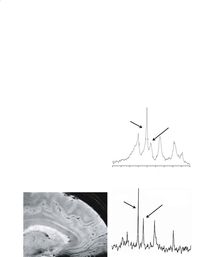
31P NMR Spectrum of Skeletal Muscle at 1.9 T

Baseline unresolved

PCr

γ-ATP

Fig. 2.2. High resolution magnetic resonance image using gradient echo acquisition at 8 T (Ohio State University)

Fig. 2.3a,b. Magnetic resonance phosphorus spectroscopy at 1.9 (a) and 9.4 T (b). The high field spectrum demonstrates improved resolution

shifts. This will be observed as an anomalous shift in position of the fat signal along the read direction in the MRI image, the chemical shift artifact. An example of this effect is shown in Fig. 2.4. The apparent shift in position of the fat signal increases with field strength and similar chemical shift artifacts can be observed for any species with a chemical shift substantially different from water. Chemical shift artifacts can, however, often be attenuated by offresonance presaturation of the nonaqueous species. In fact, on higher-field instruments, these species can often be saturated with less concomitant saturation of water as a consequence of improved spectral resolution. Other techniques for fat suppression, based on, for example, T1 relaxation time difference, are also available.

2.2.4.2

Magnetic Field Strength and Susceptibility E ects

Magnetic susceptibility, χ, refers to the relative difference between the strength of the magnetic field measured inside and outside an object composed of a specific material. In the most common case, electron shielding results in a reduction of the magnetic field within a substance so that χ is negative. These substances can be thought of as slightly repelling or excluding the external field, and are

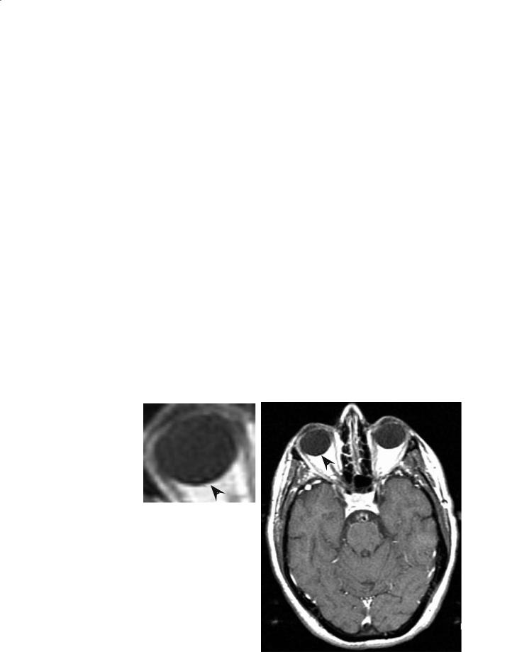
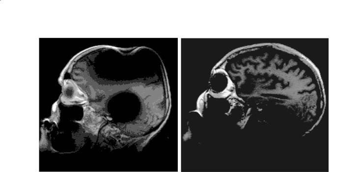
called diamagnetic. Diamagnetism is a weak effect, resulting in a reduction of the magnetic field within a diamagnetic object of at most a few parts per million (ppm). If the sample to be scanned does not have constant susceptibility, there will be variations in the actual field strength inside the sample. In general, significant B0 inhomogeneity arising from susceptibility differences will be encountered wherever there is a sudden transition in tissue composition or voids in the tissue. For example, a large difference in χ is encountered between brain tissue and pockets of air in the nasal sinuses. In this region of the brain, large distortions in B0 field strength and resulting MRI artifacts are frequently observed at air-tissue interfaces. The presence of metal prostheses or fragments in the body also results in large susceptibility differences. Even if these metal objects are not ferromagnetic, they possess a magnetic susceptibility very different from that of tissue or water and thus may cause pronounced artifacts in their immediate vicinity. An example of a typical artifact caused by variations in susceptibility is shown in Fig. 2.5. Clearly, these variations will change whenever a new sample is inserted into the magnet. Some experimental protocols, particularly in spectroscopy, require corrections for these distortions each time a new sample is inserted for scanning.

Just as the effects of chemical shift differences are magnified at higher magnetic field strength, the effects of differences in susceptibility are similarly amplified. As with chemical shift, susceptibility effects on resonance frequency scale linearly with main magnetic field strength and can result in apparent shifts in position along the read direction in MRI images. More importantly, however, differences in susceptibility within a sample cause inhomogeneities in B0 field strength which result in decreased T2*, broader linewidths and poorer resolution in spectroscopic experiments, and often pronounced imaging artifacts due to signal loss. In practice, particularly large susceptibility differences are found in regions of the body where pockets of air are present, since air has a very different susceptibility than typical tissue. Where susceptibility is exploited for image contrast, for example in some fMRI studies as well as in studies employing exogenous contrast agents, the increase in this effect at higher field may be advantageous.

2.2.4.3

Cost and Siting Considerations

For a given bore size, the higher the magnetic field strength, the greater the size, weight and cost of the magnet become. For superconducting magnets, this is largely the result of the increased number of turns of superconducting wire needed to produce a

stronger field in a given working volume. Both the wire itself and the fabrication of the magnet coils are expensive and this cost scales at least linearly with the length of wire required to build the magnet. Moreover, a larger magnet coil demands a larger, heavier cryostat to maintain the coil below its critical temperature. Lastly, as magnetic field strength increases, the internal forces felt by the coil windings increase, necessitating heavier supports and reinforcement within the magnet. The greater size and weight of high field magnets impose demands upon the design of the buildings where they are located. Not only must additional floor space be allocated for the magnet itself, but consideration must also be given to the increased volume of the fringe field (also called stray field) surrounding the magnet in all directions. The fringe field is that portion of the magnetic field that extends outside the bore of the magnet. It is desirable to minimize the dimensions of this field in order to minimize both the effects that the magnet has on objects in its surroundings (e.g., pacemakers, steel tools, magnetic cards) and also the disturbance of the main magnetic field by objects outside the magnet (e.g., passing motor vehicles, rail lines, elevators). While the extent of the fringe field can be reduced by various shielding techniques, the large fringe field of high-field magnets contributes to a need for more space when compared to lower field scanners of comparable bore size.

2.2.5

Magnet Bore Size, Orientation, and Length

In addition to field strength, a traditional, closed, cylindrical MRI magnet is characterized by its bore size. Analogously, magnets for open MRI are described by their gap size, i.e., the distance between their pole pieces. We will refer to either of these dimensions as the magnet’s bore size. It is important to note that the magnet bore size does not represent the diameter of the largest object that can be imaged in that magnet. This is due to the fact that the shim coil, gradient coil and radio-frequency probe take up space within the magnet bore,reducing the space available for the subject to be imaged. However, the magnet bore size does place constraints on the maximum inner diameters of each of these components and thus is the primary factor determining the usable diameter available for the patient. For example, a magnet bore diameter of 100 cm is common for whole-body clinical applications, while an 80 cm bore magnet typically only allows insertion of the patient’s head once the shim, gradient and radio-frequency coils are installed.

In open MRI magnets, the magnetic field direction is usually vertical and thus perpendicular to the head–foot axis of the patient. An open magnet is depicted in Fig. 2.6. This is to be contrasted with traditional MRI magnets, in which the magnetic field direction is oriented along the long axis of the subject. This difference has consequences for the design of shim, gradient and radio-frequency coils in open MRI. Note that in any magnet, the direction parallel to the B0 magnetic field is always referred to as the Z axis or axial direction while the radial direction is always perpendicular to B0.

In the design of horizontal bore magnets for clinical use, there is an emphasis on minimizing the distance from the front of the magnet cryostat to the center of the magnetic field. Shortening this distance facilitates insertion of the patient and minimizes patient discomfort. However, shortening the magnet coil length may lead to decreased B0 homogeneity, while shortening the magnet cryostat may compromise the insulation of the liquid helium bath and lead to decreased hold time.

2.2.6

Field Stability

The term field stability refers to temporal variation of the magnetic field. Instability in the B0 field from any source directly results in instability in resonance

Fig. 2.6. An open clinical magnet system. (Courtesy of Siemens)

frequency and may thus cause image or spectral artifacts and poor spectral resolution. When these variations are due to intrinsic changes within the magnet (and, for resistive electromagnets, the magnet’s power supply), the change in magnetic field strength with time is called drift.A typical specification for the maximum drift rate of a modern superconducting magnet is 0.01–0.1 ppm per hour. Superconducting magnets can also experience field instability associated with changes in the temperature of the liquid helium bath that cools the magnet coils.

Conversely, temporal changes in the magnetic field due to external disturbances, such as moving elevators or trains nearby, are called magnetic interference effects. Magnetic interference can also result from the presence of magnetic fields external to the MRI magnet, such as from large transformers, power lines and motors. External forces may also indirectly affect the magnetic field by causing vibration of the magnet coil and cryostat. For this reason as well as to support the weight of the magnet and magnetic shielding, it is common practice to locate MRI magnets on the lowest floor possible and far away from vibration-generating equipment. Clearly, elimination of external effects on the magnetic field requires careful site planning prior to system installation.

2.2.7

Magnetic Field Homogeneity

While the stability of an MRI magnet refers to the relative variation in the main magnetic field with

time,typically independent of spatial position,B0 homogeneity refers to the variation in B0 over position within the magnet’s working volume. Magnetic field homogeneity is usually expressed in units of ppm over the surface of a specific diameter spherical volume (DSV). The process of measuring the variation in magnetic field over a specified region inside the magnet is called field mapping. Spatial inhomogeneities in the B0 magnetic field can arise from a variety of sources including imperfections in the construction of the magnet itself.As noted, B0 inhomogeneity also results from variations in the magnetic susceptibility of materials within the magnet coil.

Because homogeneity of the main magnetic field over the imaging or spectroscopic volume is essential, dedicated electromagnetic coils (shim coils) are provided to optimize the B0 field homogeneity within the design of the main magnet. In a superconducting electromagnet, superconducting shims are additional coils of superconducting wire wound coaxially with the main coil in such a way as to generate specific field gradients. For each principal direction, there is typically a dedicated shim coil with an independent electrical circuit. During magnet installation, current may be independently adjusted in the main coil and each of the superconducting shim coils in order to optimize B0 homogeneity within the magnet’s working volume. Since, like the main magnet coil, these shim coils are superconducting, large currents may flow through them with no resistance and no external power supply once energized. Thus, superconducting shim coils can generate strong field gradients with high temporal stability. Readjusting the current in these coils is an infrequent operation requiring special apparatus and addition of liquid helium to the magnet.

Unlike superconducting shims, passive shims do not rely upon the flow of electrical current through a coil to generate a field gradient. Instead, they are pieces of ferromagnetic metal of a size and shape designed to improve B0 homogeneity when they are inserted into the magnet.

Magnets are also provided with room temperature shims that can be adjusted on a regular basis as needed. These can be adjusted manually or automatically to compensate for differeces in susceptibility between different patients or patient positions. Since these are resistive electromagnets, they require a stable power supply and their magnitude is limited.

Specifications for magnetic field homogeneity generally distinguish between values achieved by the unshimmed magnet and those obtained after adjusting current in the room-temperature shims. Moreover, homogeneity will be specified over smaller DSVs

for smaller bore magnets, as is appropriate for the smaller working volume of the magnet. Usually, homogeneity will be specified for two or more specific DSVs since there is no simple, reliable equation relating field homogeneity to spherical diameter about the field center. A typical field homogeneity specification for a whole-body MRI magnet with optimized roomtemperature shims might be 0.06 ppm over a 20-cm DSV and 2 ppm over a 50-cm DSV, while a small-bore research magnet might achieve 2.5 ppm over a 10-cm DSV.In evaluating these specifications,it is important to consider the size of the typical sample to be imaged and the field of view that will be employed.

2.2.8

Magnetic Field Shielding

Because high-field, large bore MRI magnets generate an extensive fringe field, they are capable of both adversely affecting nearby objects as well as experiencing interference from these objects. Since 5 G (0.5 mT) is generally regarded as the maximum safe field for public exposure, the extent of the fringe field is typically described by the dimensions of the 5-G isosurface centered about the magnet. In an unshielded cylindrical magnet,this isosurface is roughly ellipsoidal with a longer dimension along the B0 axis and a shorter radial dimension. The fringe field can be characterized by the radial and axial dimensions of the “5-G line” surrounding the magnet. In order to reduce the magnitude and extent of the fringe field and thus minimize interaction between the magnet and its environment, both passive and active shielding techniques are commonly used. Passive shielding consists of ferromagnetic material placed outside the magnet. Passive shields are generally constructed from thick plates of soft iron, an inexpensive material with relatively high magnetic permeability. In order to shield a magnet with ferromagnetic plates, the substantial attractive force between the magnet and the shielding material must be considered in the design of the magnet.Active shielding consists of one or more electromagnetic coils wound on the outside of the main magnet coil but with opposite field orientation. Typically, in a superconducting magnet, the shield coils are superconducting as well and are energized simultaneously with the main coil during installation. The field generated by the shield coils partially cancels the fringe field of the main coil, thereby reducing the fringe field dimensions. As a rule, both active and passive shielding can reduce the dimensions of the 5-G fringe field by roughly a factor

of two in each direction. This often makes it possible to site a magnet in a space too small or too close to a magnetically-sensitive object to accommodate an unshielded magnet of similar size and field strength. New MRI magnets are increasingly designed with built-in active shielding.

2.3

Pulsed Field Gradients

The function of the pulsed field gradient system in an MRI instrument is to generate linear, stable, reproducible B0 field gradients along specific directions with the shortest possible rise and fall times. While the primary use of pulsed field gradients in MRI is to establish a correspondence between spatial position and resonance frequency, gradients are also used for other purposes, such as to irreversibly dephase transverse magnetization. Gradient fields are produced by passing current through a set of wire coils located inside the magnet bore. The need for rapid switching of gradients during pulse sequences makes the design and construction of pulsed field gradient systems quite technologically demanding. The performance of a pulsed field gradient system is specified by parameters including gradient strength, linearity, stability and switching times. In addition, gradient systems are characterized by their bore size, shielding and cooling design.

2.3.1

Uses of Pulsed Field Gradients

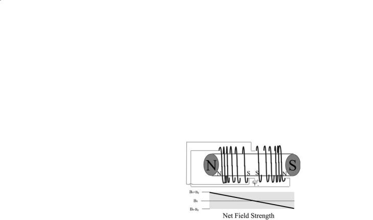
Gradient sets are designed to introduce field variation in the X, Y, and Z directions within the magnet. Thus, an X gradient is designed to produce a change in B0 directly proportional to distance along the X direction: ∆B0=Gxx, where x is the distance from the isocenter of the X gradient coil, and similarly for Y and Z. The isocenters for X, Y and Z coils should coincide exactly. Also, the gradient coil set is generally placed so that its isocenter coincides with the B0 field center. The value Gx is the X gradient strength and is typically stated in mT/m or in G/cm (1 G/ cm=10 mT/m). By causing the B0 field strength to vary linearly with X position, applying a pulsed field gradient causes the resonance frequency of each nuclear spin to depend linearly upon its X position.If we define the resonance frequency offset ∆ν to be zero for a nuclear spin at the isocenter, ∆ν=ν–νx=0 then

we have ∆ν=-γGxx/2π whenever the X gradient is switched on. For a particular nucleus, if Gx is known accurately, we can then determine the x position of that nucleus simply by measuring its frequency offset ∆ν. Similarly, by applying a frequency-selective excitation pulse in conjunction with an X gradient, we can excite nuclear spins located in a specific region along the X axis. This correspondence between B0, frequency and spatial position under the influence of field gradients forms the basis for all magnetic resonance imaging experiments and is illustrated in Fig. 2.7.

Fig. 2.7. Diagram of a solenoidal gradient coil and the effect on net magnetic field

2.3.1.1

Slice and Volume Selection Gradients

In MRI experiments, slice selection refers to the selective excitation of nuclear spins within a slab with a specific orientation, thickness, and position. This is accomplished by simultaneously applying a pulsed field gradient, called the slice gradient, and a frequency-selective radio-frequency pulse. While the slice gradient is on, the resonance frequency of each nucleus within the gradient coil depends upon its position along the slice gradient direction. The frequency offset and excitation bandwidth of the RF pulse are then set to excite nuclei with a specific range of resonance frequencies, which has the effect of exciting all nuclei located between specific positions along the slice axis. For example, the simultaneous application of a Z slice gradient and a frequency-se- lective RF pulse will excite all nuclei within a slab perpendicular to the Z axis. To a first approximation, all nuclei in the slab will be excited uniformly, regardless of their positions along the X and Y directions. The thickness of the slab excited by this gradient-RF pulse combination depends upon both the strength of the slice gradient and the excitation bandwidth of the RF pulse. The actual flip angle delivered to a group of spins with a particular resonance frequency depends