Книги по МРТ КТ на английском языке / MR Imaging in White Matter Diseases of the Brain and Spinal Cord - K Sartor Massimo Filippi Nicola De Stefano Vincent Dou

upon the shape (amplitude and phase modulation), duration, and frequency offset of the RF pulse. If all these parameters are fixed, then the excitation bandwidth is fixed and the slice thickness depends only on the inverse of slice gradient strength:

Slice thickness = 2π (Excitation Bandwidth) / γGslice

Thus, thinner slices can be imaged by increasing the slice gradient strength at a constant excitation bandwidth. While thinner slices can also be achieved by modifying the RF pulse length and shape in order to decrease the excitation bandwidth, this has several practical disadvantages, including longer minimum echo time (TE). Thus, for optimum resolution in the slice direction, it is desirable to have high slice gradient strength. Finally, note that it is possible in an MRI experiment to selectively excite a slice oriented in any direction in three-dimensional space. Slices parallel to the XY, YZ or XZ planes are termed axial (or transverse), sagittal or coronal depending upon the placement of the subject in the scanner. Slices not parallel to any of these planes are called oblique slices. Regardless of slice orientation, the slice gradient is always applied perpendicular to the desired slice plane. Gradients to select oblique slices are created by simultaneously passing current through two or three of the electromagnetic gradient coils X, Y and Z.

Applying three slice-selective gradient and RF pulse pairs in sequence selectively excites nuclei within a defined volume. Once these nuclei have been excited, sampling the resulting NMR signal yields a spectrum reflecting the chemical composition of the selected volume. Just as increased slice gradient strength permits the selection of thinner slices at fixed RF bandwidth, volume-selective NMR spectroscopy experiments gain better spatial resolution with stronger slice gradients. Alternatively, smaller volumes can be selectively excited by decreasing the bandwidth of the RF pulses, but this results in longer minimum echo time TE, and carries other disadvantages.

2.3.1.2

Read Gradients

As we have seen, when a B0 field gradient is applied along a specific axis, the resonance frequency of each nuclear spin becomes dependent on its position along that axis. Picturing each nuclear spin as giving rise to a single, sharp NMR spectral peak at a posi- tion-dependent frequency, a large ensemble of spins spread over a range of positions along the gradient

axis will give rise to a broad NMR spectrum called a profile. If the peaks from each nucleus are identical except for their center frequency, then the profile represents a histogram displaying the number of nuclei resonating at each frequency and thus located at each position along the gradient axis. Just as in a purely spectroscopic NMR experiment, during the application of the read gradient in a MRI scan, we must digitize the time-domain signal at a sufficiently fast rate to accurately measure the highest frequencies in the spectrum. Mathematically, the minimum digitization rate required to accurately sample the NMR signal for a given spectrum is given by the Nyquist condition: BW=1/DW ≥2νmax where νmax is the highest frequency in the spectrum, DW is the dwell time or time increment between successive sample points and BW is the sampling, or acquisition,bandwidth.As long as the read gradient is on, the relative resonance

frequency ∆ν of any spin is given by ∆ν=-γGreadx/2π, where x is the distance from the read gradient iso-

center and Gread is the strength of the read gradient. Combining these two relations we find that in order

to accurately measure a nuclear spin’s position along the read direction, that spin must have a distance

to isocenter no greater than π•BW/(γGread). In other words, digitizing the time-domain NMR data with a

sweep width of BW, we can only measure positions

lying in a region of width FOVread=2π•BW/(γGread) centered at the read gradient isocenter, where FOVread

is the field of view in the read gradient direction. In digitizing the time-domain NMR signal, we

select not only DW, but also the number of samples to collect in the time domain, which is equal to the number of data points in the frequency domain after Fourier transformation,and thus equal to the number of pixels in the MRI image along the read gradient di-

rection. This number of pixels, MTXread, is called the matrix size in the read dimension of the image. The

total time over which the NMR signal is digitized is

called the acquisition time: AQ = DW • MTXread. The spatial resolution, ∆xread, of the MRI image along the

read direction is simply given by FOVread/MTXread. Recalling that FOVread is given by 2π•BW/(γGread), we observe that spatial resolution in the read direction

can be minimized, for constant MTXread, by either minimizing BW or maximizing Gread. Minimizing BW

has the additional benefit of improving SNR, as we shall discuss in Sect. 2.6, but this also implies longer DW=1/BW, and hence longer AQ and a larger minimum echo time. This may not be acceptable in fast imaging experiments or in the imaging of short T2 or short T2* samples.In contrast,optimizing spatial resolution along the read direction by maximizing Gread

with fixed bandwidth has no penalties, but is limited by gradient performance. Thus, in the specification of an MRI scanner, it is relatively advantageous to have a larger maximum Gread and a larger maximum BW.

2.3.1.3

Phase Encoding Gradients

A phase encoding gradient in the pulse sequence permits spatial localization in the direction perpendicular to the read gradient direction within the slice plane. This requires multiple acquisitions with a phase encoding gradient inserted between the slice selection and read gradients. During the constant duration phase-encoding period, the nuclear spins undergo a net phase change that depends upon their position along the direction of the phase encoding gradient. This phase change is reflected in a change in the overall intensity of the NMR signal acquired during the read period. With the read and slice gradients operating as discussed above, one can construct a two-dimensional slice-selected MRI image from a sequence of acquisitions performed with incremented phase encoding gradient strength. Likewise, a three-dimensional image can be obtained by simultaneously incrementing phase encoding gradients on two different axes, both perpendicular to the read axis.

2.3.2

Gradient Linearity

As we have mentioned, both shim and pulsed field gradients are typically created by passing electrical current through wire windings. The geometry of the gradient desired determines the shape of the coil windings.

In order to be useful for spatial encoding, either in the read, phase or slice directions, a pulsed field gradient must at a minimum produce a monotonic variation of B0 with X,Y or Z position over the volume of the sample being imaged; this is needed to ensure a one-to-one mapping of B0 field strength to position. In addition, it is highly desirable that the variation of B0 with position be perfectly linear over the sample volume. If this is satisfied, then position and B0 field strength (or resonance frequency) are related by a simple linear transformation, making gradient calibration a simple matter. The term gradient linearity refers to the degree to which a gradient coil generates a perfectly linear variation of B0 with position over a certain range of distances from its isocenter.

2.3.3

Gradient Switching and Eddy Currents

While shim gradients are typically applied continuously and at constant strength, pulsed field gradients must be switched on and off rapidly and frequently during a MRI pulse sequence. This requirement, along with the need for excellent linearity and much higher gradient strength makes pulsed field gradient systems much more challenging to design and build than shim systems. Ideally, we would like to expose the nuclear spins to gradient pulses which turn on and off instantly. In practice, this is not possible due to both inductive and eddy current effects. The finite inductance of the gradient coil affects the dynamics of current and thus gradient amplitude, ∂B0/∂x, on a time scale of hundreds of microseconds. In contrast, eddy current effects influence the B0 field distribution directly on a time scale from milliseconds to seconds. Eddy currents are electrical currents induced in any conductive materials, such as the magnet bore tube, located in close proximity to the gradient coil. These induced currents are proportional to the gradient slew rate, that is, ∂B0/∂t=dG/dt and thus can be large when the gradient current rises or falls rapidly. Eddy currents flowing through these conductive materials generate a magnetic field oriented opposite in direction to ∂B0/∂t. The nuclear spins experience the sum of the magnetic fields generated by the gradient coil and eddy currents. The net effect is to lengthen both the time required to achieve a stable, usable field gradient as well as the time needed to stabilize the B0 field after the pulse ends. Depending upon the gradient slew rate and the configuration of conductive material inside and outside the gradient coil, eddy current-induced fields may cause the actual B0 distribution felt by the spins to be quite different from the intended distribution. These effects manifest themselves in both broadening and frequency shifts in NMR spectra acquired immediately after a gradient pulse, and contribute to imaging artifacts. One longstanding method of reducing eddy currents is to use gradient preemphasis, in which the input to the gradient amplifiers is calculated to produce the desired gradient in the sample, accounting for coil inductance and eddy current effects. In addition, modern gradient coils are actively shielded. Just as in the design of actively-shielded magnets, these gradient coils are equipped with shield windings which largely cancel the stray field outside the bore of the gradient set. Using a combination of the above techniques, it is possible to achieve a stable B0 field within a few hundred microseconds of the rising or falling edge

of a gradient pulse. The actual gradient switching performance of a MRI scanner is often specified by the time required after the beginning of a pulse to reach 90% or 99% of the desired gradient strength. Small microimaging gradient coils can achieve rise and fall times of 100 µs or less while gradient coils for clinical imaging typically require 200–300 µs to achieve 99% stability after gradient switching. Faster gradient switching permits shorter echo times and more rapid acquisitions, and reduces image distortions resulting from undesired time-varying contributions to the spatial distribution of B0. While these effects are noticeable in many MRI experiments, they are particularly pronounced in fast imaging sequences such as echo planar imaging (EPI). In EPI, the read and phase encoding gradients are switched on and off rapidly many times in each scan in order to sample a large number of phase-encoded steps using a train of gradient echoes. Ideally, this gradient switching can be achieved very quickly,permitting an entire two-dimensional image to be acquired in tens of milliseconds. For this to be possible, inductive and eddy current effects must be minimized so that the B0 field achieves the desired magnitude and spatial distribution quickly after each switch. When this is not the case, distortions in the B0 field result in signal loss and distortions in the images. In general, any experiment which requires frequent, rapid gradient switching will produce undistorted images only if considerable care is exercised to minimize gradient stabilization times. Thus, the gradient rise and fall times are critical specifications in the evaluation of any MRI scanner.

2.3.4

Gradient Strength

From the discussion in Sect. 2.3.1,it is clear that strong gradients permit improved in-plane spatial resolution and thinner slices. The gradient strength which is achievable in an actual MRI scanner depends upon several factors. First, just as an electromagnet can be made stronger by increasing the number of turns in the magnet coil, gradient strength can be increased by adding turns to a gradient coil. Unfortunately, this also increases the electrical resistance of the coil and thus the heat dissipated by the coil, I2R, for a given current, I. This heat must be dissipated by air or water cooling. A larger number of turns also increases the inductance of the coil, which impedes rapid gradient switching. In order to accurately set the field of view and slice thickness and to faithfully depict the

sizes and positions of features within a sample, it is necessary that the actual strength of each gradient coil be carefully calibrated. This is typically achieved by imaging an object with known dimensions. With a particular choice of field of view and slice thickness, the pulse amplitude applied to each gradient amplifier is calibrated to give the correct dimensions of the object in MRI slices taken in three orthogonal directions. It is then assumed that the required gradient current will scale linearly with the field of view or slice thickness desired in all other experiments. In other words, we assume that the gradient strength is a linear function of the gradient amplifier input voltage over the operating range of the gradient system. Since all modern gradient amplifiers are linear amplifiers, this is generally an excellent assumption.

2.3.5

Gradient Stability and Duty Cycle

In any imaging experiment, it is important that the amplitude of a gradient pulse be stable following the initial ramp-up period and be reproducible from scan to scan. Failure to meet these conditions results in image distortions for poor gradient stability and ghosting artifacts when gradient reproducibility is inadequate.

The duty cycle of any pulse-generating device is defined as the fraction of time during which the device is active,i.e.,producing an output signal,and is expressed as a percentage.A particularly high gradient duty cycle occurs in experiments requiring long echo trains, such as EPI, and when the repetition time TR is very short. In some situations, a burst of strong gradient pulses with a high short-term duty cycle is tolerable to the amplifiers provided that TR is long, so that the longterm duty cycle is low. Both the maximum duty cycle and the tendency of long gradient pulses to droop in amplitude are functions of the capacity of the gradient amplifier power supply to sustain large loads, and the gradient coil’s ability to dissipate heat.

2.4

Radio-Frequency Coils

In MRI scanners, radio-frequency transmit coils are used to transmit electromagnetic waves into a sample, creating the oscillating B1 magnetic field needed to excite the nuclear spins.In contrast,receive coils detect the weak signal emitted by the spins as they precess

in the B0 field. For typical values of the magnetic field strength B0 encountered in NMR and MRI instruments, these signals lie in the radio-frequency region of the electromagnetic spectrum. Thus, RF coils can be thought of as radio antennas. The same coil may be used for both exciting the spins and receiving the resulting NMR signal, or transmission and reception may be performed by separate coils which are carefully constructed to minimize inductive coupling between them. RF coils are characterized by the volume over which they can generate a uniform B1 field or, equivalently, receive a NMR signal with uniform gain. The most important property of a RF coil, however, is the efficiency with which it converts electromagnetic waves at the specified frequency into electric current, and vice versa. There is a reciprocity relation between the performance of the coil as a transmitter of excitation pulses and as a receiver of faint NMR signals, meaning that both can be optimized simultaneously.A variety of RF coil designs have been developed which attempt to optimize one or both of these specifications over a given volume.

2.4.1

Common RF Coil Designs

2.4.1.1

Solenoidal RF Coils

The solenoidal configuration used for magnet and shim coils is also useful for RF antennas. Driving a solenoidal coil with an alternating current generates a spatially homogeneous time varying B1 magnetic field with the same frequency as the driving current. This produces a torque on nuclear spins which are within the coil and which have a component of their orientation perpendicular to the coil axis. Thus, it is necessary that the coil produce a B1 field which is not parallel to the B0 field. Similarly, a receive coil must be able to detect a time-varying magnetic field perpendicular to B0 in order to detect a NMR signal. Since the B1 field generated by a solenoidal coil is parallel to the bore axis of the solenoid, the coil should be oriented with this axis perpendicular to B0. Consequently, solenoidal coils are primarily used for imaging in vitro samples. Solenoidal RF coils generate very homogeneous fields, especially over samples which are small in diameter and length compared to the dimensions of the solenoid. This enables them to excite and detect a NMR signal from any nuclear spins within the bore of the solenoid. Solenoids are highly efficient

as both transmitter and receiver coils and are very simple to construct.

2.4.1.2

Surface Coils and Phased Arrays

A surface coil is a loop of wire which generates or detects B1 fields along a direction perpendicular to the plane of the loop. Like solenoidal coils, surface coils are highly efficient and are easy to build. Since they have a B1 axis perpendicular to the loop plane, surface coils offer convenient access for application to a wide variety of anatomical sites while maintaining B1 perpendicular to B0. However, the RF field generated by a surface coil is very inhomogeneous, with maximum B1 magnitude in the plane of the coil and a rapid falloff in B1 with distance from this plane. Likewise, when used for detecting an NMR signal, a surface coil can only detect nuclei within a short distance from the coil plane. Specifically, when a surface coil is placed against the surface of a sample, nuclei may be excited and detected to a depth approximately equal to the diameter of the coil and over an area approximately equal to the dimensions of the coil. The small, well-defined volume over which a surface coil transmits or receives a signal makes these coils ideal for spatial localization in certain circumstances without requiring the use of field gradients. Surface coils have long been used to obtain in vivo NMR spectra of peripheral muscle, brain, heart, liver and other relatively superficial tissues with simple purely spectroscopic pulse sequences. In MRI scanners, where spatial localization can be achieved by gradients, surface coils are less often used for excitation and are instead primarily employed as high-sensitivity receive-only coils in conjunction with a large, homogeneous transmit-only resonator. The limited area over which a single surface coil can detect a NMR signal can be overcome by combining two or more surface coils to form a phased array coil. These coils must be coupled with electronic components which combine the signals from each coil into a single signal or to multiple, independent receivers. The phased array covers the surface area which a much larger surface coil would observe, but exhibits the higher sensitivity of the small coils which make up the array. Phased array coils are commonly used in clinical imaging of the spine, where an extensive field of view is required but the tissue of interest is relatively superficial. Both individual surface coils and phased arrays can be constructed with curvature to ensure close placement to a given anatomical site, thereby optimizing both sensitivity and depth of view.

26

2.4.1.3

RF Volume Resonators

When a NMR signal must be excited and detected from deep tissue or where homogeneous excitation is required and a solenoidal coil does not provide convenient patient access, a variety of RF volume resonators is available. These may be defined as cylindrical, multi-loop coils which generate a B1 field perpendicular to the bore axis. A birdcage resonator is very commonly used as a head or body coil in both clinical and animal MRI scanners (see coil in Fig. 2.1). Birdcage resonators can be used in both transmit-receive and transmit-only configurations. In the latter arrangement, a birdcage coil is used to achieve homogeneous excitation over a subject while a surface coil is used for high-sensitivity detection of the signal from a superficial region of the subject. Unlike simpler resonator designs, the birdcage resonator can be operated in quadrature mode in order to achieve an increase in B1 field strength (or, equivalently, detection sensitivity) of a factor of √2. In transmission mode, the driving current is split into two separate signals which are simultaneously applied to the birdcage resonator in order to create circularly polarized fields of equal magnitude but 90° out of phase. The vector sum of these fields is

aB1 field oriented perpendicular to the resonator’s bore axis with a magnitude √2 times as great as each component. In reception mode, a quadrature birdcage coil simultaneously detects components of B1 along two orthogonal directions, yielding two separate electrical signals which can be combined with an appropriate electronic circuit external to the resonator. The transverse electromagnetic resonator (TEM),

adesign relatively new to MRI, has become popular due to its excellent efficiency at very high frequencies, where other resonator designs offer poorer performance.TEM resonators are especially useful for brain imaging on high-field research MRI scanners.

2.4.2

Coil Characteristics and Optimization

For a coil to transmit or receive RF signals at the nuclear magnetic resonance frequency, the coil must be a component of a transmitter or receiver circuit tuned to this frequency. In addition, for efficient transfer of RF power to and from the coil, the electrical impedance of the coil must be matched to the impedance of the transmitter or receiver electronics. Tuning and matching may be achieved by manual or automatic adjustment of variable components located prefer-

K. W. Fishbein et al.

ably within the coil housing itself or alternatively in a remote enclosure.

The quality factor (Q) measures the efficiency with which the coil converts an electrical signal into ra- dio-frequency radiation or vice versa. Consequently, a coil with high Q is efficient at detecting weak radio frequency NMR signals, creating an electrical signal that may be amplified and digitized by the spectrometer’s receiver electronics. A transmitter coil having a high Q indicates that it creates a relatively strong B1 field from an alternating current of a certain amplitude. Because the pulse length τ90 needed to achieve a 90º flip angle is simply related to the magnitude of B1 by the equation γB1τ90=π/2,the coil efficiency is often specified by stating the 90º pulse length achievable for a specific amount of transmitter power applied to the coil containing a specific sample. Equivalently, coil efficiency can be stated in terms of the transmitter power needed to achieve a 90° flip angle in a given sample with an RF pulse of given duration and shape.

The term filling factor indicates the fraction of a coil’s sensitive volume that is occupied by sample. For fixed coil dimensions, quality factor Q and incident transmitter power, the filling factor has minimal effect on the 90º pulse length and the coil’s efficiency for exciting the nuclear spins. However, filling factor has a strong effect on sensitivity when detecting a NMR signal, with higher filling factor corresponding to higher sensitivity. For a sample of fixed dimensions, it is advantageous to use the smallest coil that will accommodate the region of the sample to be imaged while providing acceptable RF homogeneity over that region. Using the smallest possible receive coil size also minimizes the amount of sample noise which will be detected along with the NMR signal and thus maximizes signal-to-noise ratio. Because, in practice, it is not possible to achieve both high filling factor and high RF homogeneity with a single transmit/receive coil, it is not uncommon to use a large resonator for homogeneous excitation of the nuclei and a much smaller surface or phased array coil to detect the NMR signal with optimum filling factor, minimum noise pickup and thus maximum SNR. As we described earlier, this crossed coil configuration requires careful adjustment of geometry and synchronization of tuning and detuning to prevent crosstalk between the transmit-only resonator and the receive-only surface coil or coils.

In principle, it is possible to make τ90 as short as desired by simply increasing the transmitter power delivered to the coil, even if the transmit coil has low Q. MRI instruments are typically equipped with radio

frequency amplifiers delivering kilowatts of power at the NMR frequency and it is very desirable for transmitter coils to be able to operate safely at high power. The ability of a coil to withstand high power pulses depends both on the amplitude of these pulses and their duty cycle. When a coil is exposed to high incident transmitter power, even for a relatively short duration, very large voltages may be created across components such as capacitors and closely-spaced conductors, leading to dielectric breakdown and arcing. Conversely, exposure to long pulses at high power may lead to excessive resistive heating and subsequent failure of inductors and resistive conductors. Just as dissipation of heat within the transmitter coil and associated components imposes a limit on RF power levels and duty cycle in a MRI experiment, care must be taken not to produce excessive heating of the sample, typically an animal or human subject. When exposed to RF radiation,tissue undergoes heating depending upon its dielectric constant. This heat is dissipated largely by blood circulation, which carries heat from deep within the body to the skin and extremities for radiative cooling. When the RF power level and duty cycle are sufficiently low, this cooling mechanism prevents tissue temperatures from rising excessively. Common safety practice is based upon limiting any temperature rise in tissue to one degree Celsius during a MRI examination. In order to satisfy regulatory guidance, MRI experiments performed on living subjects must not exceed certain limits on specific absorption rate (SAR). Power deposition is in general a greater problem at higher field strengths.

2.5 Transmitters

The term transmitter refers to the assembly of electronic components in an MRI scanner which provides an electrical signal to the transmitter coil to excite the nuclear spins. The transmitter system can be divided into low-power components, which create pulsed alternating current signals with defined timing, phase and amplitude modulation, and highpower components, which faithfully amplify this low-level signal and couple it to the transmitter coil. In modern instruments, the low-level RF electronics consist mostly or entirely of digital components while the high-power section of the transmitter is largely analog in design due to the power limitations of available digital components. Accordingly, specifications for the low-power section of an MRI transmitter are

based on clock rates and digital resolution of digi- tal-to-analog converters (DACs). In contrast, highpower transmitter subsystems are characterized by the standard amplification specifications of gain, linearity and stability as well as by their power and duty cycle limits. Additional considerations essential for MRI include slew rate, a measure of the speed with which the output of the amplifier can change, and blanking performance, the ability of the amplifier to provide zero output during signal acquisition.

The frequency range of the transmitter must be broad. In proton MRI, for example, the ability to access a wide frequency range about the nominal proton NMR frequency is desirable for several reasons. As we have discussed, it is often desirable to minimize slice thickness by maximizing slice gradient strength rather than by decreasing RF excitation bandwidth, since the latter results in increased echo time and signal losses due to relaxation. Greater slice gradient strength implies a larger dispersion of NMR frequencies along the slice direction. In addition, in order to excite slices anywhere along this direction, the transmitter must be able to generate a wide range of radio frequencies to correspond to different slabs along the slice gradient. For both proton NMR and heteronuclear (i.e., nonproton) experiments, it is desirable to have the capability to study nuclei across their entire chemical shift range. In addition, it is important to be able to excite a variety of nuclei with different gyromagnetic ratios, and hence widely different frequencies.

In addition to setting the frequency, duration and amplitude of an RF pulse, the low-power transmitter system of an MRI scanner must be capable of adjusting the phase of the pulse. By altering the phase relationship between the RF excitation pulse and the receiver reference signal, it is possible to reduce certain artifacts associated with imperfect flip angles, unwanted spin echoes, receiver imbalances and other effects. This technique, called phase cycling, causes the desired signal components to add with each scan while undesired components are subtracted from the accumulated signal.

Once the transmitter’s low-power electronics have synthesized a pulsed, amplitude modulated RF signal with the appropriate frequencies and phases, this signal must be amplified to provide sufficient power for spin excitation. High power pulses are needed in NMR and MRI in order to achieve desired flip angles with short pulse durations. In clinical MRI scanners, amplifiers up to 15–25 kW are commonly used. In each case, the RF power required to achieve the desired flip angles with adequately short pulse lengths depends upon the efficiency of the coil at the NMR frequency.

The linearity of the high-power RF amplifier refers to its ability to amplify a signal by a constant factor, that is, with constant gain, over a wide range of input amplitudes. This permits the low-power waveform which is input into the transmitter amplifier system to be faithfully reproduced as a high-power RF excitation pulse. Therefore, it is desirable to have a highpower RF amplifier with minimum variation in gain over the widest possible input amplitude range.

2.6

Radio-Frequency Receiver

After nuclear spins in a sample have been excited by RF pulses, they precess in the main magnetic field as they relax back to equilibrium. This precession induces very small voltages in the receiver coil; this signal can be on the order of microvolts. It is the function of the MRI scanner’s receiver train to greatly amplify this signal, filter out unwanted frequency components, separate real and imaginary components and digitize these components for storage and processing by the host computer. The initial amplification occurs at the natural precession frequency of the nuclei using one or more preamplifier stages. In order to help protect these very sensitive preamplifiers from overload and damage by the high-power transmitter pulses as well as to isolate the weak NMR signal from the transmitter pulse ringdown signal, MRI scanners contain a transmit-receive switch. When a single transmit-receive coil is used, the transmit-receive switch alternately connects the coil circuit to the transmitter for spin excitation and to the receiver train for signal detection, amplification, and digitization.

Together, the real and imaginary parts of the NMR signal can be thought of as a complex function with a magnitude and phase at each instant of time. Upon Fourier transformation, this phase-sensitive data yields a spectrum with both positive and negative frequencies centered about the reference frequency. This technique of obtaining a complex, phase-sensi- tive audio frequency signal by splitting and mixing with phase-shifted reference signals is known as quadrature detection.

Oncequadraturedetectionhasbeenperformed,the real and imaginary signals are further amplified and passed through low-pass filters. These filters are set to remove any components with frequencies greater

than the spectral width to be digitally sampled. This step is necessary to eliminate any signal components at frequencies too high to be properly digitized with the selected digitization rate, thus preventing highfrequency noise or unwanted resonances from being folded into the digitized signal. Ideally, the low-pass filters should present no attenuation to signal components below the cutoff frequency while totally eliminating any component above this frequency. For any real analog filter, there will always be some attenuation and phase shift as one approaches the cutoff frequency. Thus, the filters are set to a frequency somewhat higher than the full spectral width. This ensures that any resonance occurring within the selected spectral width will receive no significant attenuation from the filters.

Once the NMR signal has been amplified, mixed down to audio frequency and separated into real and imaginary components, it is digitized for computer processing. The ability to digitize rapidly allows one to achieve short echo times in fast imaging and studies of samples with rapid T2 relaxation. Consequently, maximum sampling rate is an important specification for any analog-to-digital converter (ADC), or “digitizer”. Just as important is the digital resolution of the ADC. This is the number of bits with which the digitizer represents the amplitude of the signal. It is desirable to amplify the analog signal to be digitized so that it fills as much as possible of the dynamic range, or maximum input amplitude, of the digitizer without exceeding this range. There is a tradeoff in digitizer design between speed and digital resolution. For example, a common 16-bit digitizer can sample the NMR signal at a rate of up to 2 MHz, or 0.5 µs per point, while a 10 MHz digitizer may have a digital resolution of only 12 bits. High digital resolution is advantageous in detecting small spectroscopic peaks in the presence of a much larger peak, as in NMR spectroscopy of metabolites in dilute aqueous solution.A typical MRI scanner is equipped with a 16-bit digitizer with a maximum sampling rate of at least 1 MHz.

Once the NMR signal has been digitized, it may be subjected to a variety of digital signal conditioning procedures. Digital signal processing (DSP) is generally performed by a dedicated microprocessor rather than by the scanner’s host computer and the processed signal is accumulated in a dedicated buffer memory. This greatly increases the rate at which data may be accumulated and prevents data loss due to interruptions in data transmission or host computer CPU availability.

CONTENTS

3.1Introduction 29

3.2.1Image Encoding 29 3.2.1.1 Slice Selection 29 3.2.1.2 Frequency Encoding 30 3.2.1.3 Phase encoding 30

3.2.2Single Spin-Echo 30

3.2.3Multi-Echo Spin-Echo 32

3.3Gradient-Echo Imaging 32

3.3.1Spoiled Gradient-Echo 34

3.3.2Refocused Gradient-Echo 34

3.3.3Magnetization-Prepared Gradient-Echo 34

3.4Inversion Recovery 35

3.5Artifacts 37

3.5.1Metal Artifacts 37

3.5.2 Chemical Shift Artifacts 37

3.5.3Motion Artifacts 37

3.5.4Wrap-Around Artifacts 38

3.1 Introduction

In Chap. 1 the fundamental behaviors of a single spin, or of a group of spins, were discussed. In brief summary, after the spins are aligned in a polarizing magnetic field, it is possible to add energy and to cause them to acquire transverse magnetization while giving up longitudinal magnetization. The recovery of longitudinal magnetization and the decay of transverse magnetization are characterized by relaxation times. Signal arises from the transverse component of magnetization and the interaction of that transverse magnetization with the conductors of the radiofrequency (RF) coil, due to Faraday induction. Certain types of signal loss (dephasing) can be

D. L. Kraitchman, VMD, PhD

Associate Professor, Johns Hopkins University, School of Medicine, Department of Radiology, Division of MR Research, 601 N. Caroline Street, Office 4231, Baltimore, MD 21287-0845, USA

reversed by a refocusing pulse to form a spin echo, which is advantageous in that its signal is relatively strong. In this chapter we begin with the MR signal and the spin echo, and develop the construction of images using combinations of RF pulses and application of gradients.

3.2

The Spin-Echo Pulse Sequence

3.2.1

Image Encoding

3.2.1.1

Slice Selection

In order to examine only a specific slice in the body rather than exciting the entire body with an RF pulse, a gradient magnetic field is superimposed on the external field, B0, during the application of the RF pulse. This external and additional magnetic field is applied with variable intensity as a function of location. Specifically, the gradient field, as well as the total field that is the sum of the B0 and the gradient, increases from the center of the magnet outward in the positive direction, and decreases in the opposite direction. This establishes a characteristic field strength, and thus, resonance frequency, for each position along the gradient axis.

The thickness of the slice can be selected in two ways. One method is by changing the range of RF pulse frequencies or bandwidth. A smaller range of RF frequencies, such as 64–64.5 mHz, will resonate protons in a thinner slice than a larger range of frequencies, such as 64–65 mHz.

Another method of changing the slice thickness is by modifying the slope or the gradient field.A steeper gradient, i.e., one that has a larger variation in field strength, will cause frequency precession to vary to a larger degree and enable a thinner slice selection.

30

3.2.1.2

Frequency Encoding

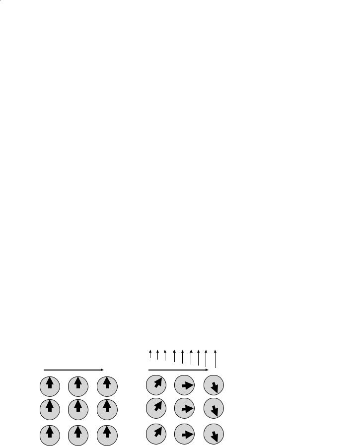
By applying a gradient during the RF pulse, one can select a slice or position in the body as well as the thickness of this slice. If we apply another gradient field during the acquisition of the signal, each position along the gradient direction will be associated by the Larmor relationship with a unique resonance frequency, and the spins at that position will precess according to that frequency.For example,if the gradient pulse is applied along x and increases from the left to right side of the body, then the precession frequency will also increase from left to right (Fig. 3.1). Thus, a one-to-one correspondence between frequency and spatial position is created by using an externally applied magnetic field gradient. Because this gradient creates a relationship between spatial location and frequency, it is called the frequency encoding gradient. A one-dimensional (1D) Fourier transform (FT) of the recorded signal will yield signal amplitudes at different frequencies which correspond to the spatial location in 1D. Note that frequency encoding is not sufficient to uniquely determine the two-dimensional (2D) location within the slice since all protons in one column will have the same frequency. The frequency encoding gradient is often referred to as the read or readout gradient since it is applied during data acquisition or read-out.

3.2.1.3

Phase encoding

In order to discriminate between points within the same column after frequency encoding, we apply

D. L. Kraitchman

another gradient at 90º (or orthogonal) to the frequency encoding gradient. This gradient is called the phase encoding gradient. The phase encoding gradient is applied for a brief period of time, typically prior to the frequency encoding gradient, and causes a change in the frequency of precession for a brief period of time. During the gradient operation, proton spins precess in accordance with the altered magnetic field, and acquire phase angles that are specifically attributable to that field. When the gradient is turned off, the frequency of precession returns to the equilibrium value, but the phase of rotation of the protons is locked in. Thus, when the gradient is turned off, each column (from the previous example) will have a different phase. This is known as phase encoding. Clearly, the magnitude of the phase change is proportional to the magnitude of the phase encoding gradient. By using both frequency and phase encoding gradients, the protons are labeled with both a frequency and phase so that 2D spatial localization can be performed.

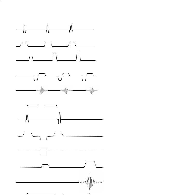
Typically, one spin echo is acquired for each gradient magnitude of phase encoding. This simple but powerful form of MR imaging is called the spin-warp pulse sequence and is diagrammed in Fig. 3.2.

3.2.2

Single Spin-Echo

The spin-echo pulse sequence is widely used in clinical practice due to the ease of implementation and the ease of varying parameters that will alter MR contrast based on differences in tissue T1, T2, or proton density. The spin-echo pulse sequence (Fig. 3.3)

Fig. 3.1. Initially the net magnetization at each pixel is aligned with the magnetic field gradient, B0, as shown for nine representative pixels. Application of the frequency encoding gradient, a linearly varying magnetic field gradient, causes an increased or decreased frequency at each pixel in proportion to the increased or decreased applied field. One dimensional localization can be performed. However, no distinction between pixels in the same column can be made because they are at the same frequency

Spinand Gradient-Echo Imaging

TE/2

180º

90º

TE

in its simplest form consists of a series of alternating 90º and 180º RF pulses. The 90º RF pulse tips the magnetization such that all the individual spins are in phase (Fig. 3.4). However, because of inhomogeneities in the magnetic field (T2* effects) dephasing of the spins will occur in addition to the dephasing caused by spin–spin interactions (true T2). The application of a 180º rephasing pulse at some time delay after application of the initial 90º RF pulse nutates

RF

Slice

Phase

Readout

the spins such that spins that were precessing more rapidly are now rotating behind the spins that were precessing more slowly (Fig. 3.4). Thus, after an identical time delay, the slower spins have caught up with the faster spins such that the spins are rephased and the spin echo is created (Fig. 3.4). This time between the initial 90º RF pulse and the moment of rephasing when read-out is performed is called the echo time (TE). The time between the application of the 90º